|
|
4 weeks ago | |
|---|---|---|
| README_files | 4 weeks ago | |
| logistic-regressor-scratch | 4 weeks ago | |
| README.md | 4 weeks ago | |
README.md
Development of a Modular Python Library from Scratch for Automated ROI Segmentation in Thermal Images
Module 2: Logistic Regressor From Scratch
Author: Sofia Samaniego Lopez
Institution: Universidad Autonoma de Baja California (UABC)
Advisor: Dr. Gerardo Marx Chavez Campos
This notebook presents Module 2 of the library's development: the implementation of a Logistic Regression Classifier from scratch.
To ensure a deep understanding of the underlying mechanics, this module avoids high-level machine learning "black-box" libraries. Instead, it builds the optimization algorithm using fundamental mathematical operations via NumPy. It covers the definition of the Sigmoid activation function, the formulation of the Log-Loss (Cross-Entropy) cost function, and the iterative optimization of weights using Gradient Descent.
The classic Iris dataset is utilized to evaluate the model's capacity to estimate probabilities and establish a linear decision boundary for binary classification based on morphological features.
1. Environment Setup & Data Loading
Importing core libraries for data manipulation (pandas), mathematical operations (numpy), and visualization (matplotlib). The Iris dataset is loaded to extract the target variables.
!pip3 install pandas
!pip3 install numpy
!pip3 install matplotlib

import pandas as pd
import numpy as np
import matplotlib.pyplot as plt
Requirement already satisfied: pandas in c:\Users\sofia\Logistic-Regressor-From_Scratch\.venv\Lib\site-packages (3.0.3)
Requirement already satisfied: numpy>=2.3.3 in c:\Users\sofia\Logistic-Regressor-From_Scratch\.venv\Lib\site-packages (from pandas) (2.5.0)
Requirement already satisfied: python-dateutil>=2.8.2 in c:\Users\sofia\Logistic-Regressor-From_Scratch\.venv\Lib\site-packages (from pandas) (2.9.0.post0)
Requirement already satisfied: tzdata in c:\Users\sofia\Logistic-Regressor-From_Scratch\.venv\Lib\site-packages (from pandas) (2026.2)
Requirement already satisfied: six>=1.5 in c:\Users\sofia\Logistic-Regressor-From_Scratch\.venv\Lib\site-packages (from python-dateutil>=2.8.2->pandas) (1.17.0)
Requirement already satisfied: numpy in c:\Users\sofia\Logistic-Regressor-From_Scratch\.venv\Lib\site-packages (2.5.0)
Requirement already satisfied: matplotlib in c:\Users\sofia\Logistic-Regressor-From_Scratch\.venv\Lib\site-packages (3.11.0)
Requirement already satisfied: contourpy>=1.0.1 in c:\Users\sofia\Logistic-Regressor-From_Scratch\.venv\Lib\site-packages (from matplotlib) (1.3.3)
Requirement already satisfied: cycler>=0.10 in c:\Users\sofia\Logistic-Regressor-From_Scratch\.venv\Lib\site-packages (from matplotlib) (0.12.1)
Requirement already satisfied: fonttools>=4.22.0 in c:\Users\sofia\Logistic-Regressor-From_Scratch\.venv\Lib\site-packages (from matplotlib) (4.63.0)
Requirement already satisfied: kiwisolver>=1.3.1 in c:\Users\sofia\Logistic-Regressor-From_Scratch\.venv\Lib\site-packages (from matplotlib) (1.5.0)
Requirement already satisfied: numpy>=1.25 in c:\Users\sofia\Logistic-Regressor-From_Scratch\.venv\Lib\site-packages (from matplotlib) (2.5.0)
Requirement already satisfied: packaging>=20.0 in c:\Users\sofia\Logistic-Regressor-From_Scratch\.venv\Lib\site-packages (from matplotlib) (26.2)
Requirement already satisfied: pillow>=9 in c:\Users\sofia\Logistic-Regressor-From_Scratch\.venv\Lib\site-packages (from matplotlib) (12.2.0)
Requirement already satisfied: pyparsing>=3 in c:\Users\sofia\Logistic-Regressor-From_Scratch\.venv\Lib\site-packages (from matplotlib) (3.3.2)
Requirement already satisfied: python-dateutil>=2.7 in c:\Users\sofia\Logistic-Regressor-From_Scratch\.venv\Lib\site-packages (from matplotlib) (2.9.0.post0)
Requirement already satisfied: six>=1.5 in c:\Users\sofia\Logistic-Regressor-From_Scratch\.venv\Lib\site-packages (from python-dateutil>=2.7->matplotlib) (1.17.0)
df = pd.read_csv('iris_basic.csv')
df
| sl | sw | pl | pw | target | tNames | |
|---|---|---|---|---|---|---|
| 0 | 5.1 | 3.5 | 1.4 | 0.2 | 0 | setosa |
| 1 | 4.9 | 3.0 | 1.4 | 0.2 | 0 | setosa |
| 2 | 4.7 | 3.2 | 1.3 | 0.2 | 0 | setosa |
| 3 | 4.6 | 3.1 | 1.5 | 0.2 | 0 | setosa |
| 4 | 5.0 | 3.6 | 1.4 | 0.2 | 0 | setosa |
| ... | ... | ... | ... | ... | ... | ... |
| 145 | 6.7 | 3.0 | 5.2 | 2.3 | 2 | virginica |
| 146 | 6.3 | 2.5 | 5.0 | 1.9 | 2 | virginica |
| 147 | 6.5 | 3.0 | 5.2 | 2.0 | 2 | virginica |
| 148 | 6.2 | 3.4 | 5.4 | 2.3 | 2 | virginica |
| 149 | 5.9 | 3.0 | 5.1 | 1.8 | 2 | virginica |
150 rows × 6 columns
2. Binary Classification Setup & Data Visualization
Extracting the 'Petal Width' (pw) as the independent feature (x) and the target class (y).
x = df['pw'].to_numpy().reshape(-1, 1)
y = df['target'].to_numpy().reshape(-1, 1)

# Convert target to binary: 1 if setosa (class 0), 0 otherwise
y = (y==0).astype(float)
# Adding visual noise (Jitter) to observe point density
yJitter = y+np.random.uniform(-0.2,0.2,size=y.shape)
plt.plot(x,yJitter,'og', alpha=0.1)
plt.show()
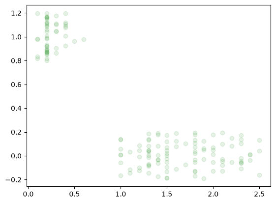
Understanding the Jitter Plot:
In binary classification, true labels are strictly 0 or 1. If plotted directly, data points overlap perfectly, masking the true density of the samples. By adding uniform random noise (jitter) to the y-axis, the points spread out vertically, allowing us to visually inspect the data distribution and density for both classes.
3. The Sigmoid Activation Function
The mathematical core of logistic regression. Linear regression outputs continuous values from -\infty to +\infty. The Sigmoid function smoothly maps any real-valued number into a probability range bounded between 0 and 1.
Formula:
\sigma(z) = \frac{1}{1+e^{-z}}(Note: np.clip is used to bound extreme values and prevent overflow errors during exponential calculation).
def sigmoid(z):
    sig= 1/(1+np.exp(-z))
    return sig
xNew = np.linspace(-5,5,100)
model = sigmoid(xNew)
plt.plot(xNew,model)
plt.plot(x,yJitter,'og', alpha=0.1)
plt.show()
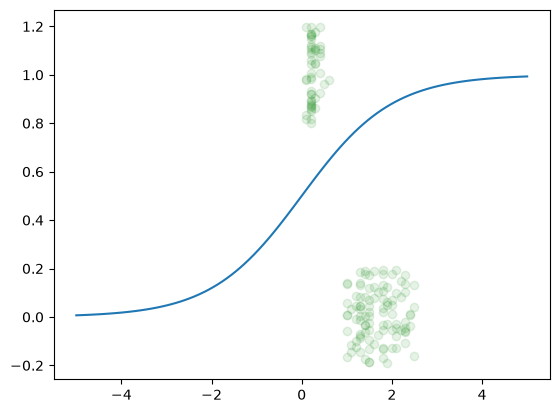
This plot illustrates the model's core activation function alongside the empirical distribution of the Iris dataset.
- Sigmoid Activation Curve: The green line represents the non-linear transformation
\sigma(z) = \frac{1}{1+e^{-z}}. This function maps input features into a probability space between0and1, providing the mathematical foundation for the model's confidence levels. - Data Distribution (Jittered): The green markers represent the actual feature values. As binary classes are constrained to
\{0, 1\}, random vertical noise (jitter) is applied to the data points to prevent overlap, revealing the density and separation between the two classes.
By overlaying the Sigmoid curve on the jittered data, we can visually inspect how well the model's probability estimates align with the observed class clusters.
def sigmoid(z):
    # Clip limits z to avoid exp overflow
    z = np.clip(z, -500, 500)
    sig= 1/(1+np.exp(-z))
    return sig
4. Cost Function: Log-Loss (Cross-Entropy)
This function calculates the error between the model's predicted probabilities (p) and the true binary labels (y).
Probabilities are clipped using a tiny epsilon (\epsilon) to prevent mathematical undefined errors (like \log(0)), which would break the algorithm.
def logLoss(y, p, eps=1e-12):
    p = np.clip(p, eps, 1-eps)
    loss = -np.mean(y*np.log(p) + (1-y)*np.log(1-p))
    return loss
5. Model Training via Gradient Descent
Instead of solving an equation directly, the model learns iteratively.
- Initialization: Random weights (
\theta_0for bias,\theta_1for the feature) are generated. - Forward Pass: Predictions are computed using the dot product and the Sigmoid function.
- Gradient Calculation: The error gradient is calculated across all samples.
- Update: Weights are adjusted in the opposite direction of the gradient, scaled by the learning rate (
lr).
lr = 0.2
epochs = 1000

# Add a column of ones to X for the bias term (intercept)
X = np.column_stack([np.ones_like(x), x])
m = X.shape[0]

# Random weight initialization
theta = np.random.rand(2,1)
theta
array([[0.83841703],
       [0.1412671 ]])
# Training loop
for i in range(epochs):
   z = X @ theta
   h = sigmoid(z) # Predicted probability

   # Gradient computation and weight update
   grad = X.T @ (h-y) / m
   theta -= lr * grad

theta0, theta1 = theta[0,0], theta[1,0]
print(f"Optimized Bias (Theta 0): {theta0}")
print(f"Optimized Weight (Theta 1): {theta1}")
Optimized Bias (Theta 0): 4.309159539504179
Optimized Weight (Theta 1): -6.028218019470694
6. Inference and Decision Boundary Visualization
Functions to compute continuous probabilities and absolute binary classes based on a 0.5 threshold.
def predictProba(x, theta0, theta1):
    x = np.array(x, float).reshape(-1)
    model = sigmoid(theta0 + theta1 * x)
    return model

def predict(x, theta0, theta1, thresh=0.5):
    model = (predictProba >= thresh).astype(int)
    # Returns 1 if probability >= threshold, else 0
# Plotting the empirical data alongside the optimized Sigmoid curve
xNew = np.linspace(0,2.5,100)
p = predictProba(xNew, theta0, theta1)
plt.plot(xNew, p, ':g')
plt.plot(x,yJitter,'og', alpha=0.1)
plt.show()
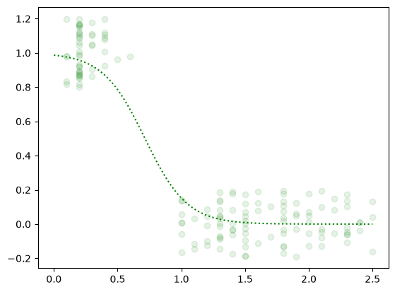
Understanding the Final Plot:
The green dotted line represents the trained Sigmoid curve. It illustrates the model's probability estimation across different Petal Widths. Where the curve crosses the 0.5 probability mark on the y-axis, the model sets its hard mathematical boundary, switching its classification verdict from Class 0 to Class 1.