# Data Gattering
```python
import time
import numpy as np
import tclab
```
```python
```
```python
n = 300
t = np.linspace(0,n-1,n)
T1 = np.empty_like(t)
with tclab.TCLab() as lab:
lab.Q1(40)
for i in range(n):
T1[i] = lab.T1
print(T1[i])
time.sleep(1)
```
TCLab version 1.0.0
Arduino Leonardo connected on port /dev/cu.usbmodem1301 at 115200 baud.
TCLab Firmware 2.0.1 Arduino Leonardo/Micro.
24.218
23.154
24.347
24.411
24.411
24.347
24.314
24.347
24.347
23.896
24.476
24.637
24.669
24.669
25.056
25.088
24.991
25.088
25.217
25.281
25.313
25.668
25.668
25.636
26.022
25.926
19.126
26.248
26.248
26.055
25.152
26.699
26.989
26.957
27.021
27.118
27.247
27.344
27.666
27.183
27.795
27.892
28.021
28.311
28.214
28.504
28.536
28.762
28.826
28.858
29.245
29.181
29.374
29.6
29.567
29.793
29.761
29.89
30.147
30.147
30.438
30.599
30.728
30.856
30.76
31.018
31.114
31.34
31.533
31.501
31.727
31.469
32.017
32.081
32.113
32.5
32.403
32.403
32.693
32.726
32.887
33.016
33.048
33.08
33.37
33.37
33.499
33.725
33.789
33.821
34.047
34.079
34.144
34.305
34.434
34.434
34.659
34.756
34.659
34.691
34.917
34.981
34.981
35.271
35.4
35.336
35.239
35.594
35.626
35.819
26.796
35.948
27.408
36.174
35.304
36.271
36.528
36.561
36.689
36.657
36.979
36.979
37.044
37.205
37.173
37.237
37.205
37.302
37.656
37.56
37.592
37.882
37.882
37.817
38.043
37.173
38.269
38.365
38.397
38.591
33.016
26.022
38.913
38.945
38.913
38.945
38.945
39.235
39.203
39.268
39.3
39.493
39.042
39.59
39.622
39.654
39.815
39.88
39.912
39.912
40.009
40.009
40.234
40.234
40.234
40.363
40.524
40.524
40.557
40.557
40.653
40.814
40.557
40.911
40.879
41.072
41.169
41.104
41.072
41.104
41.137
41.523
41.33
41.523
41.523
41.62
41.813
41.781
41.846
41.813
41.942
42.136
42.136
42.136
42.136
42.104
42.168
42.361
42.458
42.232
42.49
42.361
42.394
42.426
42.394
42.716
42.748
42.813
42.651
42.813
42.748
42.941
43.103
43.135
43.103
43.038
43.135
43.264
43.425
43.328
43.328
43.457
43.457
43.521
43.683
43.779
43.683
43.683
43.715
43.973
43.94
44.102
44.005
44.005
44.005
44.23
44.359
44.424
44.392
44.327
44.327
44.424
44.521
43.779
44.682
44.714
44.649
44.649
44.746
44.778
44.907
44.972
42.2
44.939
45.036
44.907
44.327
43.876
45.004
45.197
45.294
45.358
45.326
45.229
45.358
45.101
45.423
45.391
45.713
45.681
45.616
45.713
45.616
45.713
45.713
45.713
45.745
45.648
45.971
45.938
45.938
45.938
46.067
45.971
46.035
46.132
46.196
45.938
46.164
46.261
46.261
46.229
46.261
46.229
46.229
46.357
46.551
46.519
46.551
46.583
TCLab disconnected successfully.
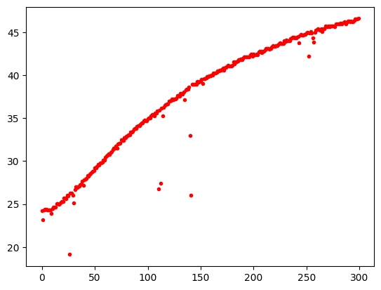
```python
import matplotlib.pyplot as plt
plt.plot(T1, '.r')
plt.show()
```
```python
import pandas as pd
DF = pd.DataFrame(T1)
DF.to_csv("data.csv", index=False)
```
# Linear regression
The linear regression is a training procedure based on a linear model. The model makes a prediction by simply computing a weighted sum of the input features, plus a constant term called the bias term (also called the intercept term):
$$ \hat{y}=\theta_0 x_0 + \theta_1 x_1 + \theta_2 x_2 + \cdots + \theta_n x_n$$
This can be writen more easy by using vector notation form for $m$ values. Therefore, the model will become:
$$
\begin{bmatrix}
\hat{y}^0 \\
\hat{y}^1\\
\hat{y}^2\\
\vdots \\
\hat{y}^m
\end{bmatrix}
=
\begin{bmatrix}
1 & x_0^0 & x_1^0 & \cdots x_n^0\\
1 & x_0^1 & x_1^1 & \cdots x_n^1\\
\vdots & \vdots \\
1 & x_0^m & x_1^m & \cdots x_n^m
\end{bmatrix}
\begin{bmatrix}
\theta_0 \\
\theta_1 \\
\theta_2 \\
\vdots \\
\theta_n
\end{bmatrix}
$$
Resulting:
$$\hat{y}= h_\theta(x) = x \theta $$
**Now that we have our mode, how do we train it?**
Please, consider that training the model means adjusting the parameters to reduce the error or minimizing the cost function. The most common performance measure of a regression model is the Mean Square Error (MSE). Therefore, to train a Linear Regression model, you need to find the value of θ that minimizes the MSE:
$$ MSE(X,h_\theta) = \frac{1}{m} \sum_{i=1}^{m} \left(\hat{y}^{(i)}-y^{(i)} \right)^2$$
$$ MSE(X,h_\theta) = \frac{1}{m} \sum_{i=1}^{m} \left( x^{(i)}\theta-y^{(i)} \right)^2$$
$$ MSE(X,h_\theta) = \frac{1}{m} \left( x\theta-y \right)^T \left( x\theta-y \right)$$
# The normal equation
To find the value of $\theta$ that minimizes the cost function, there is a closed-form solution that gives the result directly. This is called the **Normal Equation**; and can be find it by derivating the *MSE* equation as a function of $\theta$ and making it equals to zero:
$$\hat{\theta} = (X^T X)^{-1} X^{T} y $$
$$ Temp = \theta_0 + \theta_1 * t $$
```python
import pandas as pd
df = pd.read_csv('data.csv')
df
```
|
0 |
| 0 |
24.218 |
| 1 |
23.154 |
| 2 |
24.347 |
| 3 |
24.411 |
| 4 |
24.411 |
| ... |
... |
| 295 |
46.357 |
| 296 |
46.551 |
| 297 |
46.519 |
| 298 |
46.551 |
| 299 |
46.583 |
300 rows × 1 columns
```python
import numpy as np
y = df['0']
n = 300
t = np.linspace(0,n-1,n)
X = np.c_[np.ones(len(t)), t]
X
```
array([[ 1., 0.],
[ 1., 1.],
[ 1., 2.],
[ 1., 3.],
[ 1., 4.],
[ 1., 5.],
[ 1., 6.],
[ 1., 7.],
[ 1., 8.],
[ 1., 9.],
[ 1., 10.],
[ 1., 11.],
[ 1., 12.],
[ 1., 13.],
[ 1., 14.],
[ 1., 15.],
[ 1., 16.],
[ 1., 17.],
[ 1., 18.],
[ 1., 19.],
[ 1., 20.],
[ 1., 21.],
[ 1., 22.],
[ 1., 23.],
[ 1., 24.],
[ 1., 25.],
[ 1., 26.],
[ 1., 27.],
[ 1., 28.],
[ 1., 29.],
[ 1., 30.],
[ 1., 31.],
[ 1., 32.],
[ 1., 33.],
[ 1., 34.],
[ 1., 35.],
[ 1., 36.],
[ 1., 37.],
[ 1., 38.],
[ 1., 39.],
[ 1., 40.],
[ 1., 41.],
[ 1., 42.],
[ 1., 43.],
[ 1., 44.],
[ 1., 45.],
[ 1., 46.],
[ 1., 47.],
[ 1., 48.],
[ 1., 49.],
[ 1., 50.],
[ 1., 51.],
[ 1., 52.],
[ 1., 53.],
[ 1., 54.],
[ 1., 55.],
[ 1., 56.],
[ 1., 57.],
[ 1., 58.],
[ 1., 59.],
[ 1., 60.],
[ 1., 61.],
[ 1., 62.],
[ 1., 63.],
[ 1., 64.],
[ 1., 65.],
[ 1., 66.],
[ 1., 67.],
[ 1., 68.],
[ 1., 69.],
[ 1., 70.],
[ 1., 71.],
[ 1., 72.],
[ 1., 73.],
[ 1., 74.],
[ 1., 75.],
[ 1., 76.],
[ 1., 77.],
[ 1., 78.],
[ 1., 79.],
[ 1., 80.],
[ 1., 81.],
[ 1., 82.],
[ 1., 83.],
[ 1., 84.],
[ 1., 85.],
[ 1., 86.],
[ 1., 87.],
[ 1., 88.],
[ 1., 89.],
[ 1., 90.],
[ 1., 91.],
[ 1., 92.],
[ 1., 93.],
[ 1., 94.],
[ 1., 95.],
[ 1., 96.],
[ 1., 97.],
[ 1., 98.],
[ 1., 99.],
[ 1., 100.],
[ 1., 101.],
[ 1., 102.],
[ 1., 103.],
[ 1., 104.],
[ 1., 105.],
[ 1., 106.],
[ 1., 107.],
[ 1., 108.],
[ 1., 109.],
[ 1., 110.],
[ 1., 111.],
[ 1., 112.],
[ 1., 113.],
[ 1., 114.],
[ 1., 115.],
[ 1., 116.],
[ 1., 117.],
[ 1., 118.],
[ 1., 119.],
[ 1., 120.],
[ 1., 121.],
[ 1., 122.],
[ 1., 123.],
[ 1., 124.],
[ 1., 125.],
[ 1., 126.],
[ 1., 127.],
[ 1., 128.],
[ 1., 129.],
[ 1., 130.],
[ 1., 131.],
[ 1., 132.],
[ 1., 133.],
[ 1., 134.],
[ 1., 135.],
[ 1., 136.],
[ 1., 137.],
[ 1., 138.],
[ 1., 139.],
[ 1., 140.],
[ 1., 141.],
[ 1., 142.],
[ 1., 143.],
[ 1., 144.],
[ 1., 145.],
[ 1., 146.],
[ 1., 147.],
[ 1., 148.],
[ 1., 149.],
[ 1., 150.],
[ 1., 151.],
[ 1., 152.],
[ 1., 153.],
[ 1., 154.],
[ 1., 155.],
[ 1., 156.],
[ 1., 157.],
[ 1., 158.],
[ 1., 159.],
[ 1., 160.],
[ 1., 161.],
[ 1., 162.],
[ 1., 163.],
[ 1., 164.],
[ 1., 165.],
[ 1., 166.],
[ 1., 167.],
[ 1., 168.],
[ 1., 169.],
[ 1., 170.],
[ 1., 171.],
[ 1., 172.],
[ 1., 173.],
[ 1., 174.],
[ 1., 175.],
[ 1., 176.],
[ 1., 177.],
[ 1., 178.],
[ 1., 179.],
[ 1., 180.],
[ 1., 181.],
[ 1., 182.],
[ 1., 183.],
[ 1., 184.],
[ 1., 185.],
[ 1., 186.],
[ 1., 187.],
[ 1., 188.],
[ 1., 189.],
[ 1., 190.],
[ 1., 191.],
[ 1., 192.],
[ 1., 193.],
[ 1., 194.],
[ 1., 195.],
[ 1., 196.],
[ 1., 197.],
[ 1., 198.],
[ 1., 199.],
[ 1., 200.],
[ 1., 201.],
[ 1., 202.],
[ 1., 203.],
[ 1., 204.],
[ 1., 205.],
[ 1., 206.],
[ 1., 207.],
[ 1., 208.],
[ 1., 209.],
[ 1., 210.],
[ 1., 211.],
[ 1., 212.],
[ 1., 213.],
[ 1., 214.],
[ 1., 215.],
[ 1., 216.],
[ 1., 217.],
[ 1., 218.],
[ 1., 219.],
[ 1., 220.],
[ 1., 221.],
[ 1., 222.],
[ 1., 223.],
[ 1., 224.],
[ 1., 225.],
[ 1., 226.],
[ 1., 227.],
[ 1., 228.],
[ 1., 229.],
[ 1., 230.],
[ 1., 231.],
[ 1., 232.],
[ 1., 233.],
[ 1., 234.],
[ 1., 235.],
[ 1., 236.],
[ 1., 237.],
[ 1., 238.],
[ 1., 239.],
[ 1., 240.],
[ 1., 241.],
[ 1., 242.],
[ 1., 243.],
[ 1., 244.],
[ 1., 245.],
[ 1., 246.],
[ 1., 247.],
[ 1., 248.],
[ 1., 249.],
[ 1., 250.],
[ 1., 251.],
[ 1., 252.],
[ 1., 253.],
[ 1., 254.],
[ 1., 255.],
[ 1., 256.],
[ 1., 257.],
[ 1., 258.],
[ 1., 259.],
[ 1., 260.],
[ 1., 261.],
[ 1., 262.],
[ 1., 263.],
[ 1., 264.],
[ 1., 265.],
[ 1., 266.],
[ 1., 267.],
[ 1., 268.],
[ 1., 269.],
[ 1., 270.],
[ 1., 271.],
[ 1., 272.],
[ 1., 273.],
[ 1., 274.],
[ 1., 275.],
[ 1., 276.],
[ 1., 277.],
[ 1., 278.],
[ 1., 279.],
[ 1., 280.],
[ 1., 281.],
[ 1., 282.],
[ 1., 283.],
[ 1., 284.],
[ 1., 285.],
[ 1., 286.],
[ 1., 287.],
[ 1., 288.],
[ 1., 289.],
[ 1., 290.],
[ 1., 291.],
[ 1., 292.],
[ 1., 293.],
[ 1., 294.],
[ 1., 295.],
[ 1., 296.],
[ 1., 297.],
[ 1., 298.],
[ 1., 299.]])
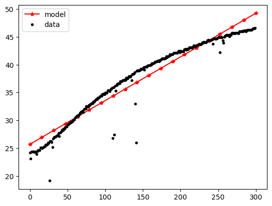
```python
theta = np.linalg.inv(X.T.dot(X)).dot(X.T).dot(y)
theta
```
array([25.70275643, 0.07850281])
```python
import matplotlib.pyplot as plt
Xnew1 = np.linspace(0,300, 20)
Xnew = np.c_[np.ones(len(Xnew1)), Xnew1]
Xnew
```
array([[ 1. , 0. ],
[ 1. , 15.78947368],
[ 1. , 31.57894737],
[ 1. , 47.36842105],
[ 1. , 63.15789474],
[ 1. , 78.94736842],
[ 1. , 94.73684211],
[ 1. , 110.52631579],
[ 1. , 126.31578947],
[ 1. , 142.10526316],
[ 1. , 157.89473684],
[ 1. , 173.68421053],
[ 1. , 189.47368421],
[ 1. , 205.26315789],
[ 1. , 221.05263158],
[ 1. , 236.84210526],
[ 1. , 252.63157895],
[ 1. , 268.42105263],
[ 1. , 284.21052632],
[ 1. , 300. ]])
```python
ypre = Xnew.dot(theta)
plt.plot(Xnew1, ypre, '*-r', label='model')
plt.plot(t,y, '.k', label='data')
plt.legend()
plt.show()
```
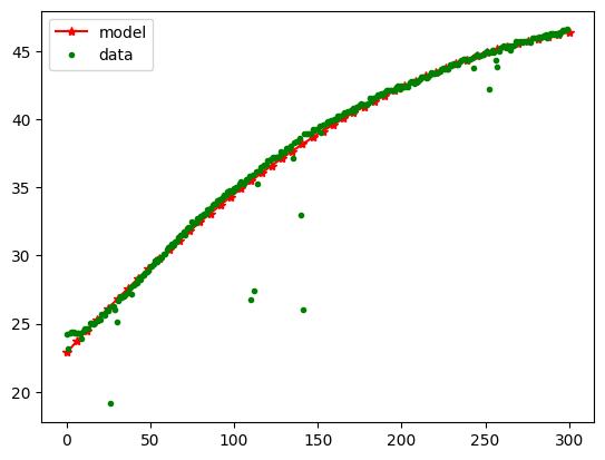
# Polynomial model
$$ Temp = \theta_0 + \theta_1 * t + \theta_2 * t^2$$
```python
X = np.c_[np.ones(len(t)), t, t*t]
theta = np.linalg.inv(X.T.dot(X)).dot(X.T).dot(y)
theta
```
array([ 2.28848082e+01, 1.35240024e-01, -1.89756565e-04])
```python
Xnew1 = np.linspace(0,300,50)
Xnew = np.c_[np.ones(len(Xnew1)), Xnew1, Xnew1*Xnew1]
ypred = Xnew.dot(theta)
plt.plot(Xnew1, ypred, '*-r', label='model')
plt.plot(t,y, '.g', label='data')
plt.legend()
plt.show()
```
# Batch Gradient Descent
$$\theta_{new} = \theta_{old}-\eta \nabla_{\theta} $$
$$\nabla_{\theta} = \frac{2}{m} X^T (X \theta -y) $$
```python
y = np.array(df['0']).reshape(300,1)
n = 300
t = np.linspace(0,n-1,n)
X = np.c_[np.ones(len(t)), t]
y
```
array([[24.218],
[23.154],
[24.347],
[24.411],
[24.411],
[24.347],
[24.314],
[24.347],
[24.347],
[23.896],
[24.476],
[24.637],
[24.669],
[24.669],
[25.056],
[25.088],
[24.991],
[25.088],
[25.217],
[25.281],
[25.313],
[25.668],
[25.668],
[25.636],
[26.022],
[25.926],
[19.126],
[26.248],
[26.248],
[26.055],
[25.152],
[26.699],
[26.989],
[26.957],
[27.021],
[27.118],
[27.247],
[27.344],
[27.666],
[27.183],
[27.795],
[27.892],
[28.021],
[28.311],
[28.214],
[28.504],
[28.536],
[28.762],
[28.826],
[28.858],
[29.245],
[29.181],
[29.374],
[29.6 ],
[29.567],
[29.793],
[29.761],
[29.89 ],
[30.147],
[30.147],
[30.438],
[30.599],
[30.728],
[30.856],
[30.76 ],
[31.018],
[31.114],
[31.34 ],
[31.533],
[31.501],
[31.727],
[31.469],
[32.017],
[32.081],
[32.113],
[32.5 ],
[32.403],
[32.403],
[32.693],
[32.726],
[32.887],
[33.016],
[33.048],
[33.08 ],
[33.37 ],
[33.37 ],
[33.499],
[33.725],
[33.789],
[33.821],
[34.047],
[34.079],
[34.144],
[34.305],
[34.434],
[34.434],
[34.659],
[34.756],
[34.659],
[34.691],
[34.917],
[34.981],
[34.981],
[35.271],
[35.4 ],
[35.336],
[35.239],
[35.594],
[35.626],
[35.819],
[26.796],
[35.948],
[27.408],
[36.174],
[35.304],
[36.271],
[36.528],
[36.561],
[36.689],
[36.657],
[36.979],
[36.979],
[37.044],
[37.205],
[37.173],
[37.237],
[37.205],
[37.302],
[37.656],
[37.56 ],
[37.592],
[37.882],
[37.882],
[37.817],
[38.043],
[37.173],
[38.269],
[38.365],
[38.397],
[38.591],
[33.016],
[26.022],
[38.913],
[38.945],
[38.913],
[38.945],
[38.945],
[39.235],
[39.203],
[39.268],
[39.3 ],
[39.493],
[39.042],
[39.59 ],
[39.622],
[39.654],
[39.815],
[39.88 ],
[39.912],
[39.912],
[40.009],
[40.009],
[40.234],
[40.234],
[40.234],
[40.363],
[40.524],
[40.524],
[40.557],
[40.557],
[40.653],
[40.814],
[40.557],
[40.911],
[40.879],
[41.072],
[41.169],
[41.104],
[41.072],
[41.104],
[41.137],
[41.523],
[41.33 ],
[41.523],
[41.523],
[41.62 ],
[41.813],
[41.781],
[41.846],
[41.813],
[41.942],
[42.136],
[42.136],
[42.136],
[42.136],
[42.104],
[42.168],
[42.361],
[42.458],
[42.232],
[42.49 ],
[42.361],
[42.394],
[42.426],
[42.394],
[42.716],
[42.748],
[42.813],
[42.651],
[42.813],
[42.748],
[42.941],
[43.103],
[43.135],
[43.103],
[43.038],
[43.135],
[43.264],
[43.425],
[43.328],
[43.328],
[43.457],
[43.457],
[43.521],
[43.683],
[43.779],
[43.683],
[43.683],
[43.715],
[43.973],
[43.94 ],
[44.102],
[44.005],
[44.005],
[44.005],
[44.23 ],
[44.359],
[44.424],
[44.392],
[44.327],
[44.327],
[44.424],
[44.521],
[43.779],
[44.682],
[44.714],
[44.649],
[44.649],
[44.746],
[44.778],
[44.907],
[44.972],
[42.2 ],
[44.939],
[45.036],
[44.907],
[44.327],
[43.876],
[45.004],
[45.197],
[45.294],
[45.358],
[45.326],
[45.229],
[45.358],
[45.101],
[45.423],
[45.391],
[45.713],
[45.681],
[45.616],
[45.713],
[45.616],
[45.713],
[45.713],
[45.713],
[45.745],
[45.648],
[45.971],
[45.938],
[45.938],
[45.938],
[46.067],
[45.971],
[46.035],
[46.132],
[46.196],
[45.938],
[46.164],
[46.261],
[46.261],
[46.229],
[46.261],
[46.229],
[46.229],
[46.357],
[46.551],
[46.519],
[46.551],
[46.583]])
```python
np.random.seed(82)
eta = 0.00001 #lerning rate
n_iteration = 1000000
m = len(y)
theta = np.random.randn(2,1)*10
theta
```
array([[ 8.40650403],
[-13.57147156]])
```python
for iterations in range(n_iteration):
gradient = 2/m * X.T.dot(X.dot(theta)- y)
theta = theta - eta*gradient
theta
#array([25.70275643, 0.07850281])
#array([[25.53711216],[ 0.07933242]]) -> 42
#array([[25.53941259],[ 0.0793209 ]]) -> 82
```
array([[25.5895366 ],
[ 0.07906986]])
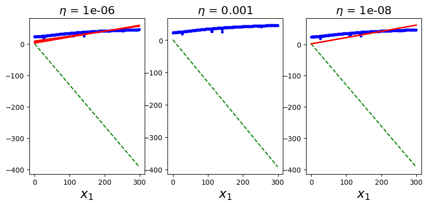
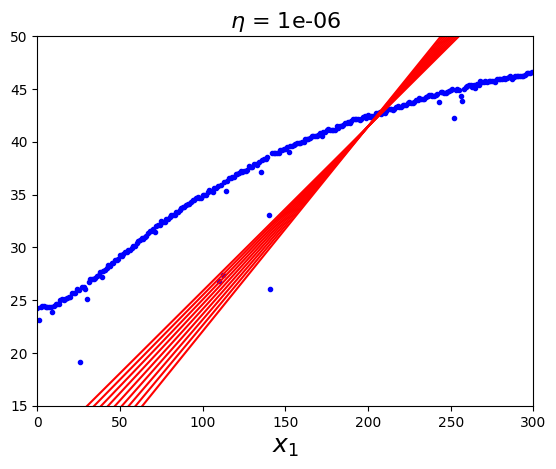
# BGD Visualization
```python
def plot_gradient_descent(eta):
m =len(y)
theta = np.random.randn(2,1)
plt.plot(t,y,'.b')
n_iteration = 1000000
Xnew1 = np.linspace(0,n-1,n)
Xnew = np.c_[np.ones(len(Xnew1)), Xnew1]
for iterations in range(n_iteration):
if iterations % 100000 == 0:
#print(iterations)
ypre = Xnew.dot(theta)
style = '-r' if iterations > 0 else 'g--'
plt.plot(Xnew1, ypre, style)
gradient = 2/m * Xnew.T.dot(Xnew.dot(theta)- y)
theta = theta - eta*gradient
plt.xlabel('$x_1$', fontsize=18)
#plt.axis([0,300, 15,50])
plt.title(r'$\eta$ = {}'.format(eta), fontsize=16)
```
```python
np.random.seed(112)
plot_gradient_descent(eta=0.000001)
theta
```
array([[25.5895366 ],
[ 0.07906986]])
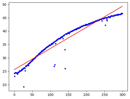
```python
plt.plot(t,y,'.b')
Xnew1 = np.linspace(0,n-1,n)
Xnew = np.c_[np.ones(len(Xnew1)), Xnew1]
ypre = Xnew.dot(theta)
plt.plot(Xnew1, ypre, '-r')
```
[]
```python
plt.figure(figsize=(10,4))
plt.subplot(131)
np.random.seed(112)
plot_gradient_descent(eta=0.000001)
plt.subplot(132)
np.random.seed(112)
plot_gradient_descent(eta=0.001)
plt.subplot(133)
np.random.seed(112)
plot_gradient_descent(eta=0.00000001)
```