10 KiB
Development of a Modular Python Library from Scratch for Automated ROI Segmentation in Thermal Images
Module 3: Artificial Neural Network (ANN)
Author: Sofia Samaniego Lopez
Institution: Universidad Autonoma de Baja California (UABC)
Advisor: Dr. Gerardo Marx Chavez Campos
This notebook presents Module 3 of the library's development: the implementation of an Artificial Neural Network (ANN) from scratch.
With the objective of maintaining algorithmic transparency and bypassing commercial "black-box" frameworks, the entire network architecture (weight matrix initialization, feedforward propagation, and backpropagation via gradient descent) has been programmed using strictly linear algebra through NumPy.
As a proof of concept and baseline evaluation, the model is trained and validated using the MNIST dataset. This demonstrates the pure mathematical algorithm's capability to classify complex patterns prior to scaling the framework for thermal image processing.
1. Environment Setup & Initialization
Importing core libraries for matrix operations and data visualization. A random seed is set to ensure reproducible weight initialization across experimental runs.
!pip3 install numpy
!pip3 install matplotlib
import numpy as np
import matplotlib.pyplot as plt
np.random.seed(12)
Requirement already satisfied: numpy in c:\Users\sofia\ANN-From-Scratch\.venv\Lib\site-packages (2.5.0)
Requirement already satisfied: matplotlib in c:\Users\sofia\ANN-From-Scratch\.venv\Lib\site-packages (3.11.0)
Requirement already satisfied: contourpy>=1.0.1 in c:\Users\sofia\ANN-From-Scratch\.venv\Lib\site-packages (from matplotlib) (1.3.3)
Requirement already satisfied: cycler>=0.10 in c:\Users\sofia\ANN-From-Scratch\.venv\Lib\site-packages (from matplotlib) (0.12.1)
Requirement already satisfied: fonttools>=4.22.0 in c:\Users\sofia\ANN-From-Scratch\.venv\Lib\site-packages (from matplotlib) (4.63.0)
Requirement already satisfied: kiwisolver>=1.3.1 in c:\Users\sofia\ANN-From-Scratch\.venv\Lib\site-packages (from matplotlib) (1.5.0)
Requirement already satisfied: numpy>=1.25 in c:\Users\sofia\ANN-From-Scratch\.venv\Lib\site-packages (from matplotlib) (2.5.0)
Requirement already satisfied: packaging>=20.0 in c:\Users\sofia\ANN-From-Scratch\.venv\Lib\site-packages (from matplotlib) (26.2)
Requirement already satisfied: pillow>=9 in c:\Users\sofia\ANN-From-Scratch\.venv\Lib\site-packages (from matplotlib) (12.2.0)
Requirement already satisfied: pyparsing>=3 in c:\Users\sofia\ANN-From-Scratch\.venv\Lib\site-packages (from matplotlib) (3.3.2)
Requirement already satisfied: python-dateutil>=2.7 in c:\Users\sofia\ANN-From-Scratch\.venv\Lib\site-packages (from matplotlib) (2.9.0.post0)
Requirement already satisfied: six>=1.5 in c:\Users\sofia\ANN-From-Scratch\.venv\Lib\site-packages (from python-dateutil>=2.7->matplotlib) (1.17.0)
2. Artificial Neural Network (ANN) Architecture
Neural Network's Basic Structure
class ann:
    #init
    def __init__():
        pass

    #feedfoward
    def feedforward():
        pass

    #backpropagation
    def backpropagation():
        pass
MyANN = ann
print(type(MyANN))
<class 'type'>
2.1 Initialization
Defining the network structure (input, hidden, and output layers). Synaptic weight matrices (W_{ih} and W_{ho}) are initialized using a normal distribution to break mathematical symmetry.
class ann:
    #init
    def __init__(self, inputNodes: int, hiddenNodes: int, outputNodes: int):
        # Nodes
        inN = inputNodes # Private var or parameters
        hN = hiddenNodes
        oN = outputNodes
        # Weights
        np.random.seed(12) #seed for reproducibility
        self.wih = np.random.randn(hN, inN) #weights for input to hidden layer
        self.who = np.random.randn(oN, hN) #weights for hidden to output layer
        pass

    #feedfoward
    def feedforward():
        pass

    #backpropagation
    def backpropagation():
        pass
MyANN = ann(3, 3, 3)
MyANN.wih
array([[ 0.47298583, -0.68142588,  0.2424395 ],
       [-1.70073563,  0.75314283, -1.53472134],
       [ 0.00512708, -0.12022767, -0.80698188]])
MyANN.who
array([[ 2.87181939, -0.59782292,  0.47245699],
       [ 1.09595612, -1.2151688 ,  1.34235637],
       [-0.12214979,  1.01251548, -0.91386915]])
2.2 Feedforward (Inference)
So the next step is to create the network of nodes and links. The most important part of the network is the link weights. They’re used to calculate the signal being fed forward, the error as it’s propagated backwards, and it is the link weights themselves that are refined in an attempt to to improve the network.
For the basic NN, the weight matrix consist of:
- A matrix that links the input and hidden layers,
Wih, of size hidden nodes by input nodes (hn×in) - and another matrix for the links between the hidden and output layers,
Who, of sizeon×hn(output nodes by hidden nodes)
X_h=W_{ih}IO_h=\sigma(X_h)Then,
X_o=W_{ho}O_{h}O_o=\sigma(X_o)class ann:
#init
def __init__(self, inputNodes: int, hiddenNodes: int, outputNodes: int):
# Nodes
inN = inputNodes # Private var or parameters
hN = hiddenNodes
oN = outputNodes
# Weights
np.random.seed(12) #seed for reproducibility
self.wih = np.random.randn(hN, inN) #weights for input to hidden layer
self.who = np.random.randn(oN, hN) #weights for hidden to output layer
pass
#feedfoward
def feedforward(self, Inputs):
# Forward pass to hidden layer
inputs = np.array(Inputs, ndmin=2).T
Xh = np.dot(self.wih, inputs)
af = lambda x: 1 / (1 + np.exp(-x))
Oh = af(Xh)
# Forward pass to output layer
Xo = self.who @ Oh
Oo = af(Xo)
return Oo
#backpropagation
def backpropagation():
pass
MyANN = ann(3, 3, 3)
MyANN.feedforward([0.1, 0.2, 0.3])
array([[0.80230104],
       [0.65960645],
       [0.48247944]])
2.3 Backpropagation (Training)
The core learning algorithm. It calculates the prediction error, propagates it backward, and dynamically updates the weight matrices using gradient descent and the chain rule.
The Gradient of Error
\frac{\partial E}{\partial w_{ho}}= -e_o\cdot \sigma \left(w_{ho} O_h\right) \left(1-\sigma\left (w_{ho} O_h\right) \right) O_h Thus,
\frac{\partial E}{\partial w_{ho}}= -e_o\cdot O_o \left(1-O_o \right) O_h class ann:
#init
def __init__(self, inputNodes: int, hiddenNodes: int, outputNodes: int):
# Nodes
inN = inputNodes # Private var or parameters
hN = hiddenNodes
oN = outputNodes
# Weights
np.random.seed(12) #seed for reproducibility
self.wih = np.random.randn(hN, inN) #weights for input to hidden layer
self.who = np.random.randn(oN, hN) #weights for hidden to output layer
pass
#feedfoward
def feedforward(self, Inputs):
# Oh
inputs = np.array(Inputs, ndmin=2).T
Xh = np.dot(self.wih, inputs)
af = lambda x: 1 / (1 + np.exp(-x))
Oh = af(Xh)
# Oo
Xo = self.who @ Oh
Oo = af(Xo)
return Oo
#backpropagation
def backpropagation(self, Inputs, Targets, Learning):
lr = Learning
inputs = np.array(Inputs, ndmin=2).T
targets = np.array(Targets, ndmin=2).T
# 1. Internal feedforward
Xh = self.wih @ inputs
af = lambda x: 1 / (1 + np.exp(-x))
Oh = af(Xh)
Xo = self.who @ Oh
Oo = af(Xo)
# 2. Error calculation
Eo = targets - Oo
Eh = self.who.T @ Eo
# 3. Weight matrices update
self.who = self.who + (lr * Eo * Oo * (1-Oo) ) @ Oh.T
self.wih = self.wih + (lr * Eh * Oh * (1-Oh) ) @ inputs.T
pass
MyANN = ann(3, 5, 3)
MyANN.backpropagation([0.1, 0.2, 0.3], [0.01, 0.01, 0.99], 0.3)
3. MNIST Dataset Exploration
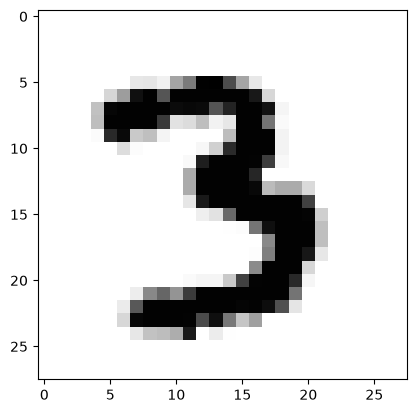
Loading the training dataset. To verify the geometric structure, a raw 784-pixel flat array is extracted and reshaped into a 28x28 2D matrix for visual confirmation.
# Load training data
file = open("mnist_train.csv")
list = file.readlines()
file.close
<function TextIOWrapper.close()>
# Visualize sample at index 120
values = list[120].split(",")
image = np.asarray(values[1:], dtype=int)
plt.imshow(image.reshape(28,28), cmap='Grays')
plt.show()
values [0]
len(list)
49999
4. Model Training
Setting up hyperparameters. During training, pixel intensities are normalized to a [0.01, 1.0] range to prevent zero-gradient issues. Target labels are formatted using an adapted One-Hot Encoding.
# hyperparameters
inputNodes = 784
hiddenNodes = 100
outNodes = 10
learningRate = 0.1
MyANN = ann(inputNodes, hiddenNodes, outNodes)
# Iterative training loop
epoch = 1
for e in range (epoch):
    for record in list:
        values = record.split(",")

        # Input data normalization
        data = np.asarray(values[1:], dtype=int)/255*0.99+0.01
        index = np.asarray(values[0],dtype=int)

        # Target Vector construction
        target = np.zeros(outNodes) + 0.01
        target[index] = 0.99

        MyANN.backpropagation(data, target, learningRate)
        pass
    pass
5. Validation & Inference
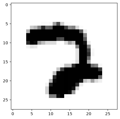
Evaluating model performance using unseen test data. A new sample is normalized and processed to extract the final prediction vector, which is then visually compared to the ground truth image.
# Load testing data
file2 = open("mnist_test.csv")
list2 = file2.readlines()
file2.close
<function TextIOWrapper.close()>
# Inference on sample 500
values = list2[500].split(",")
data = np.asarray(values[1:], dtype=int)/255*0.99+0.01

# Display probability vector for the 10 classes
MyANN.feedforward(data)
array([[1.12958417e-03],
       [7.04806122e-03],
       [1.33450332e-03],
       [9.98132913e-01],
       [1.21412650e-04],
       [6.66539345e-03],
       [2.96287176e-05],
       [1.83308214e-03],
       [8.11709452e-04],
       [1.75208890e-04]])
# Visual verification
image = np.asarray(values[1:], dtype=int)
plt.imshow(image.reshape(28,28), cmap='Grays')
plt.show()