21 KiB
Development of a Modular Python Library from Scratch for Automated ROI Segmentation in Thermal Images
Module 3: Artificial Neural Network (ANN)
Author: Sofia Samaniego Lopez
Institution: Universidad Autonoma de Baja California (UABC)
Advisor: Dr. Gerardo Marx Chavez Campos
This notebook presents Module 3 of the library's development: the implementation of an Artificial Neural Network (ANN) from scratch.
With the objective of maintaining algorithmic transparency and bypassing commercial "black-box" frameworks, the entire network architecture (weight matrix initialization, feedforward propagation, and backpropagation via gradient descent) has been programmed using strictly linear algebra through NumPy.
As a proof of concept and baseline evaluation, the model is trained and validated using the MNIST dataset. This demonstrates the pure mathematical algorithm's capability to classify complex patterns prior to scaling the framework for thermal image processing.
1. Environment Setup & Initialization
Importing core libraries for matrix operations and data visualization. A random seed is set to ensure reproducible weight initialization across experimental runs.
!pip3 install numpy
!pip3 install matplotlib
import numpy as np
import matplotlib.pyplot as plt
np.random.seed(12)
Requirement already satisfied: numpy in c:\Users\sofia\ANN-From-Scratch\.venv\Lib\site-packages (2.5.0)
Requirement already satisfied: matplotlib in c:\Users\sofia\ANN-From-Scratch\.venv\Lib\site-packages (3.11.0)
Requirement already satisfied: contourpy>=1.0.1 in c:\Users\sofia\ANN-From-Scratch\.venv\Lib\site-packages (from matplotlib) (1.3.3)
Requirement already satisfied: cycler>=0.10 in c:\Users\sofia\ANN-From-Scratch\.venv\Lib\site-packages (from matplotlib) (0.12.1)
Requirement already satisfied: fonttools>=4.22.0 in c:\Users\sofia\ANN-From-Scratch\.venv\Lib\site-packages (from matplotlib) (4.63.0)
Requirement already satisfied: kiwisolver>=1.3.1 in c:\Users\sofia\ANN-From-Scratch\.venv\Lib\site-packages (from matplotlib) (1.5.0)
Requirement already satisfied: numpy>=1.25 in c:\Users\sofia\ANN-From-Scratch\.venv\Lib\site-packages (from matplotlib) (2.5.0)
Requirement already satisfied: packaging>=20.0 in c:\Users\sofia\ANN-From-Scratch\.venv\Lib\site-packages (from matplotlib) (26.2)
Requirement already satisfied: pillow>=9 in c:\Users\sofia\ANN-From-Scratch\.venv\Lib\site-packages (from matplotlib) (12.2.0)
Requirement already satisfied: pyparsing>=3 in c:\Users\sofia\ANN-From-Scratch\.venv\Lib\site-packages (from matplotlib) (3.3.2)
Requirement already satisfied: python-dateutil>=2.7 in c:\Users\sofia\ANN-From-Scratch\.venv\Lib\site-packages (from matplotlib) (2.9.0.post0)
Requirement already satisfied: six>=1.5 in c:\Users\sofia\ANN-From-Scratch\.venv\Lib\site-packages (from python-dateutil>=2.7->matplotlib) (1.17.0)
2. Artificial Neural Network (ANN) Architecture
Neural Network's Basic Structure
class ann:
    #init
    def __init__():
        pass

    #feedfoward
    def feedforward():
        pass

    #backpropagation
    def backpropagation():
        pass
MyANN = ann
print(type(MyANN))
<class 'type'>
2.1 Initialization
Defining the network structure (input, hidden, and output layers). Synaptic weight matrices (W_{ih} and W_{ho}) are initialized using a normal distribution to break mathematical symmetry.
class ann:
    #init
    def __init__(self, inputNodes: int, hiddenNodes: int, outputNodes: int):
        # Nodes
        inN = inputNodes # Private var or parameters
        hN = hiddenNodes
        oN = outputNodes
        # Weights
        np.random.seed(12) #seed for reproducibility
        self.wih = np.random.randn(hN, inN) #weights for input to hidden layer
        self.who = np.random.randn(oN, hN) #weights for hidden to output layer
        pass

    #feedfoward
    def feedforward():
        pass

    #backpropagation
    def backpropagation():
        pass
MyANN = ann(3, 3, 3)
MyANN.wih
array([[ 0.47298583, -0.68142588,  0.2424395 ],
       [-1.70073563,  0.75314283, -1.53472134],
       [ 0.00512708, -0.12022767, -0.80698188]])
MyANN.who
array([[ 2.87181939, -0.59782292,  0.47245699],
       [ 1.09595612, -1.2151688 ,  1.34235637],
       [-0.12214979,  1.01251548, -0.91386915]])
2.2 Feedforward (Inference)
So the next step is to create the network of nodes and links. The most important part of the network is the link weights. They’re used to calculate the signal being fed forward, the error as it’s propagated backwards, and it is the link weights themselves that are refined in an attempt to to improve the network.
For the basic NN, the weight matrix consist of:
- A matrix that links the input and hidden layers,
Wih, of size hidden nodes by input nodes (hn×in) - and another matrix for the links between the hidden and output layers,
Who, of sizeon×hn(output nodes by hidden nodes)
X_h=W_{ih}IO_h=\sigma(X_h)Then,
X_o=W_{ho}O_{h}O_o=\sigma(X_o)class ann:
#init
def __init__(self, inputNodes: int, hiddenNodes: int, outputNodes: int):
# Nodes
inN = inputNodes # Private var or parameters
hN = hiddenNodes
oN = outputNodes
# Weights
np.random.seed(12) #seed for reproducibility
self.wih = np.random.randn(hN, inN) #weights for input to hidden layer
self.who = np.random.randn(oN, hN) #weights for hidden to output layer
pass
#feedfoward
def feedforward(self, Inputs):
# Forward pass to hidden layer
inputs = np.array(Inputs, ndmin=2).T
Xh = np.dot(self.wih, inputs)
af = lambda x: 1 / (1 + np.exp(-x))
Oh = af(Xh)
# Forward pass to output layer
Xo = self.who @ Oh
Oo = af(Xo)
return Oo
#backpropagation
def backpropagation():
pass
MyANN = ann(3, 3, 3)
MyANN.feedforward([0.1, 0.2, 0.3])
array([[0.80230104],
       [0.65960645],
       [0.48247944]])
2.3 Backpropagation (Training)
The core learning algorithm. It calculates the prediction error, propagates it backward, and dynamically updates the weight matrices using gradient descent and the chain rule.
Mathematical Derivation of the Cost Function and Gradient
To thoroughly understand the network's learning mechanics, we must derive the gradient of the error with respect to the synaptic weights. This procedure uses the Chain Rule from calculus and establishes the mathematical foundation for the Gradient Descent optimization strategy used in our backpropagation algorithm.
1. The Cost Function (SSE)
We define the Total Error (E) using the Sum of Squared Errors:
E = \frac{1}{2} \sum (T - O_o)^2Where T represents the target label and O_o is the predicted output. We define the output error as e_o = (T - O_o).
2. The Chain Rule Application
To update the weight matrix w_{ho} (connecting the hidden layer to the output layer), we need to determine how a change in w_{ho} impacts the total error E. We calculate the partial derivative using the Chain Rule:
\frac{\partial E}{\partial w_{ho}} = \frac{\partial E}{\partial O_o} \cdot \frac{\partial O_o}{\partial X_o} \cdot \frac{\partial X_o}{\partial w_{ho}}(Note: X_o = w_{ho} \cdot O_h represents the raw signal entering the output node before activation).
3. Solving the Partial Derivatives
- Error derivative: How the total error changes with respect to the final output.
\frac{\partial E}{\partial O_o} = -(T - O_o) = -e_o - Activation derivative: The derivative of the Sigmoid activation function
\sigma(X_o).\frac{\partial O_o}{\partial X_o} = \sigma(X_o)(1 - \sigma(X_o)) = O_o(1 - O_o) - Weight derivative: How the raw input
X_ochanges with respect to the weight matrixw_{ho}. This evaluates directly to the output of the preceding hidden layerO_h.\frac{\partial X_o}{\partial w_{ho}} = O_h
4. Final Gradient Equation
Multiplying these individual derivatives yields the final gradient of the error for w_{ho}:
\frac{\partial E}{\partial w_{ho}}= -e_o\cdot \sigma \left(w_{ho} O_h\right) \left(1-\sigma\left (w_{ho} O_h\right) \right) O_hThus, by substituting the activated output O_o, we arrive at the simplified expression:
\frac{\partial E}{\partial w_{ho}}= -e_o\cdot O_o \left(1-O_o \right) O_hThis precise formulation dictates the weight update rule programmed in our backpropagation method, scaled by the learning rate (\eta) to ensure stable convergence:
w_{ho_{new}} = w_{ho} + \eta \cdot e_o \cdot O_o(1 - O_o) \cdot O_h^Tclass ann:
#init
def __init__(self, inputNodes: int, hiddenNodes: int, outputNodes: int):
# Nodes
inN = inputNodes # Private var or parameters
hN = hiddenNodes
oN = outputNodes
# Weights
np.random.seed(12) #seed for reproducibility
self.wih = np.random.randn(hN, inN) #weights for input to hidden layer
self.who = np.random.randn(oN, hN) #weights for hidden to output layer
pass
#feedfoward
def feedforward(self, Inputs):
# Oh
inputs = np.array(Inputs, ndmin=2).T
Xh = np.dot(self.wih, inputs)
af = lambda x: 1 / (1 + np.exp(-x))
Oh = af(Xh)
# Oo
Xo = self.who @ Oh
Oo = af(Xo)
return Oo
#backpropagation
def backpropagation(self, Inputs, Targets, Learning):
lr = Learning
inputs = np.array(Inputs, ndmin=2).T
targets = np.array(Targets, ndmin=2).T
# 1. Internal feedforward
Xh = self.wih @ inputs
af = lambda x: 1 / (1 + np.exp(-x))
Oh = af(Xh)
Xo = self.who @ Oh
Oo = af(Xo)
# 2. Error calculation
Eo = targets - Oo
Eh = self.who.T @ Eo
# 3. Weight matrices update
self.who = self.who + (lr * Eo * Oo * (1-Oo) ) @ Oh.T
self.wih = self.wih + (lr * Eh * Oh * (1-Oh) ) @ inputs.T
pass
MyANN = ann(3, 5, 3)
MyANN.backpropagation([0.1, 0.2, 0.3], [0.01, 0.01, 0.99], 0.3)
3. MNIST Dataset Exploration
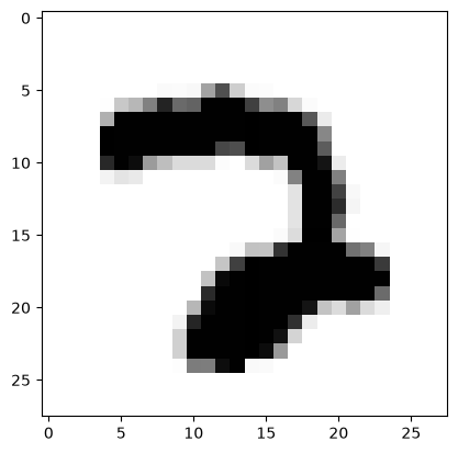
Loading the training dataset. To verify the geometric structure, a raw 784-pixel flat array is extracted and reshaped into a 28x28 2D matrix for visual confirmation.
# Load training data
file = open("mnist_train.csv")
list = file.readlines()
file.close
<function TextIOWrapper.close()>
# Visualize sample at index 120
values = list[120].split(",")
image = np.asarray(values[1:], dtype=int)
plt.imshow(image.reshape(28,28), cmap='Grays')
plt.show()
values [0]
len(list)
49999
4. Model Training
Setting up hyperparameters. During training, pixel intensities are normalized to a [0.01, 1.0] range to prevent zero-gradient issues. Target labels are formatted using an adapted One-Hot Encoding.
# hyperparameters
inputNodes = 784
hiddenNodes = 100
outNodes = 10
learningRate = 0.1
MyANN = ann(inputNodes, hiddenNodes, outNodes)
# Iterative training loop
epochs = 5
for e in range(epochs):
    total_loss = 0
    for record in list:
        values = record.split(",")

        # Input data normalization
        data = np.asarray(values[1:], dtype=int)/255*0.99+0.01
        index = np.asarray(values[0],dtype=int)

        # Target Vector construction
        target = np.zeros(outNodes) + 0.01
        target[index] = 0.99

        # Calculate loss before updating weights
        output = MyANN.feedforward(data)
        # Using SSE formulation: 0.5 * sum((target - output)^2)
        loss = np.sum(0.5 * (target.reshape(-1, 1) - output)**2)
        total_loss += loss

        # Train
        MyANN.backpropagation(data, target, learningRate)

    average_loss = total_loss / len(list)
    print(f"Epoch {e+1}/{epochs} - Average Loss: {average_loss:.4f}")
Epoch 1/5 - Average Loss: 0.0972
Epoch 2/5 - Average Loss: 0.0559
Epoch 3/5 - Average Loss: 0.0461
Epoch 4/5 - Average Loss: 0.0403
Epoch 5/5 - Average Loss: 0.0361
5. Validation & Inference
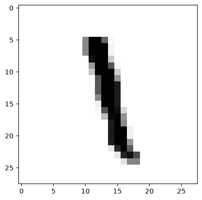
Evaluating model performance using unseen test data. A new sample is normalized and processed to extract the final prediction vector, which is then visually compared to the ground truth image.
# Load testing data
file2 = open("mnist_test.csv")
list2 = file2.readlines()
file2.close
<function TextIOWrapper.close()>
#Test Set Evaluation (Network Score)
scorecard = []

for record in list2:
    values = record.split(",")
    correct_label = int(values[0])

    # Normalize input
    data = np.asarray(values[1:], dtype=float) / 255.0 * 0.99 + 0.01

    # Get network prediction
    outputs = MyANN.feedforward(data)
    # The index of the highest value corresponds to the predicted class
    predicted_label = np.argmax(outputs)

    # Append 1 if correct, 0 if incorrect
    if predicted_label == correct_label:
        scorecard.append(1)
    else:
        scorecard.append(0)

scorecard_array = np.asarray(scorecard)
accuracy = scorecard_array.sum() / scorecard_array.size
print(f"Network Accuracy (Score) on Test Set: {accuracy * 100:.2f}%")
Network Accuracy (Score) on Test Set: 95.27%
# Inference on sample 500
values = list2[700].split(",")
data = np.asarray(values[1:], dtype=int)/255*0.99+0.01

# Display probability vector for the 10 classes
MyANN.feedforward(data)
array([[3.92210113e-05],
       [9.64025823e-01],
       [1.22524901e-03],
       [1.47886768e-02],
       [1.61851002e-03],
       [3.98689305e-03],
       [7.74585782e-05],
       [2.65175424e-03],
       [4.98386616e-03],
       [2.37478194e-03]])
# Visual verification
image = np.asarray(values[1:], dtype=int)
plt.imshow(image.reshape(28,28), cmap='Grays')
plt.show()
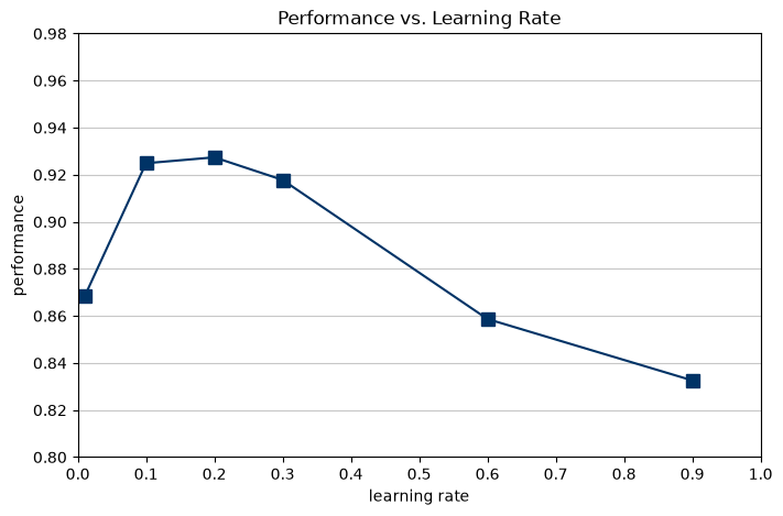
6.1 Hyperparameter Tuning: Learning Rate Impact
To optimize the network's performance, we evaluate the impact of the Learning Rate (\eta) on the final classification accuracy. The network is trained across a sweep of different learning rates [0.01, 0.1, 0.2, 0.3, 0.6, 0.9] while keeping the hidden nodes constant (100 nodes).
The results are plotted to identify the optimal step size for the Gradient Descent algorithm, avoiding both slow convergence (values too close to 0) and divergent oscillations (values too close to 1).
# 6. Hyperparameter Tuning: Learning Rate Sweep
learning_rates = [0.01, 0.1, 0.2, 0.3, 0.6, 0.9]
performances = []
hidden_nodes_baseline = 100

print("Starting Learning Rate sweep. This may take a few minutes...")

for lr in learning_rates:
    print(f"Training network with Learning Rate: {lr}...")
    # Initialize a fresh network for each test
    testANN = ann(784, hidden_nodes_baseline, 10)

    # Train 1 epoch
    for record in list:
        values = record.split(",")
        data = np.asarray(values[1:], dtype=float) / 255.0 * 0.99 + 0.01
        target = np.zeros(10) + 0.01
        target[int(values[0])] = 0.99
        testANN.backpropagation(data, target, lr)

    # Evaluate on the Test Set
    score = 0
    for record in list2:
        values = record.split(",")
        correct_label = int(values[0])
        data = np.asarray(values[1:], dtype=float) / 255.0 * 0.99 + 0.01

        outputs = testANN.feedforward(data)
        if np.argmax(outputs) == correct_label:
            score += 1

    # Calculate performance (accuracy as a decimal between 0 and 1)
    performance = score / len(list2)
    performances.append(performance)
    print(f"Performance for LR {lr}: {performance:.4f}\n")

# Plotting the exact graph requested
plt.figure(figsize=(8, 5))
plt.plot(learning_rates, performances, marker='s', markersize=8, color='#003366', linewidth=1.5)

# Formatting to match the requested style
plt.title("Performance vs. Learning Rate")
plt.xlabel("learning rate")
plt.ylabel("performance")

# Setting axes limits and ticks
plt.xlim(0, 1)
plt.xticks(np.arange(0, 1.1, 0.1))
plt.ylim(0.8, 0.98)
plt.yticks(np.arange(0.8, 1.0, 0.02))

# Adding horizontal grid lines
plt.grid(axis='y', linestyle='-', alpha=0.7)

plt.show()
Starting Learning Rate sweep. This may take a few minutes...
Training network with Learning Rate: 0.01...
Performance for LR 0.01: 0.8683

Training network with Learning Rate: 0.1...
Performance for LR 0.1: 0.9249

Training network with Learning Rate: 0.2...
Performance for LR 0.2: 0.9274

Training network with Learning Rate: 0.3...
Performance for LR 0.3: 0.9178

Training network with Learning Rate: 0.6...
Performance for LR 0.6: 0.8587

Training network with Learning Rate: 0.9...
Performance for LR 0.9: 0.8326
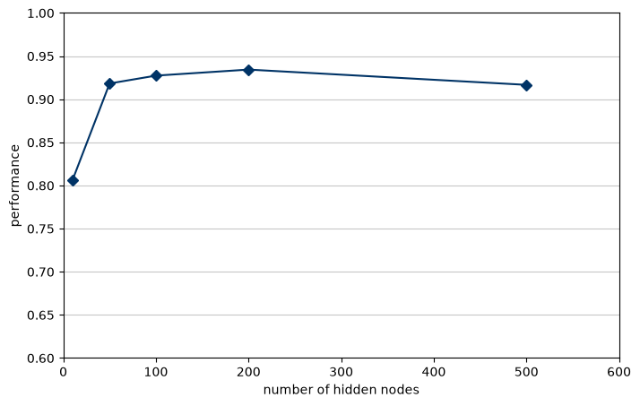
6.2 Hyperparameter Tuning: Hidden Nodes Capacity
In this experiment, we evaluate the effect of the network's capacity by varying the number of hidden nodes [10, 50, 100, 200, 500]. The Learning Rate is kept constant at 0.2.
The resulting curve demonstrates the law of diminishing returns in neural network architecture. While increasing the number of nodes initially provides a massive boost in classification performance, the accuracy plateaus after approximately 200 nodes. Beyond this threshold, adding more nodes significantly increases computational cost and memory footprint without yielding proportional accuracy gains.
# 6.2 Hyperparameter Tuning: Hidden Nodes Sweep
hidden_nodes_options = [10, 50, 100, 200, 500]
performances_hn = []
optimal_lr = 0.2 # Fixed learning rate from previous experiment

print("Starting Hidden Nodes sweep. This will take a while...")

for hn in hidden_nodes_options:
    print(f"Training network with {hn} hidden nodes...")
    testANN = ann(784, hn, 10)

    # Train 1 epoch
    for record in list:
        values = record.split(",")
        data = np.asarray(values[1:], dtype=float) / 255.0 * 0.99 + 0.01
        target = np.zeros(10) + 0.01
        target[int(values[0])] = 0.99
        testANN.backpropagation(data, target, optimal_lr)

    # Evaluate on the Test Set
    score = 0
    for record in list2:
        values = record.split(",")
        correct_label = int(values[0])
        data = np.asarray(values[1:], dtype=float) / 255.0 * 0.99 + 0.01

        outputs = testANN.feedforward(data)
        if np.argmax(outputs) == correct_label:
            score += 1

    # Calculate performance
    performance = score / len(list2)
    performances_hn.append(performance)
    print(f"Performance for {hn} nodes: {performance:.4f}\n")

# Plotting the exact graph requested
plt.figure(figsize=(8, 5))
# marker='D' creates the diamond shapes seen in the reference image
plt.plot(hidden_nodes_options, performances_hn, marker='D', markersize=6, color='#003366', linewidth=1.5)

# Formatting axes
plt.xlabel("number of hidden nodes")
plt.ylabel("performance")

# Setting axes limits and ticks to match the image
plt.xlim(0, 600)
plt.xticks(np.arange(0, 601, 100))
plt.ylim(0.6, 1.0)
plt.yticks(np.arange(0.6, 1.05, 0.05))

# Adding horizontal grid lines
plt.grid(axis='y', linestyle='-', alpha=0.7)

plt.show()
Starting Hidden Nodes sweep. This will take a while...
Training network with 10 hidden nodes...
Performance for 10 nodes: 0.8064

Training network with 50 hidden nodes...
Performance for 50 nodes: 0.9183

Training network with 100 hidden nodes...
Performance for 100 nodes: 0.9274

Training network with 200 hidden nodes...
Performance for 200 nodes: 0.9344

Training network with 500 hidden nodes...
Performance for 500 nodes: 0.9167
7. Model Selection and Architecture Evaluation
Which is the best ANN and how do you select which network is better? The best network is the one that achieves the highest accuracy on the Test Set while keeping the Cost Function (Loss) to a minimum, without falling into Overfitting. It is selected by comparing different combinations of hyperparameters (Hidden nodes and Learning Rate), evaluating them with data the network never saw during training. The winning network is the one that best generalizes to new data, not the one that memorizes the training data.
8. Microcontroller Deployment Strategy
How do we implement it on a microcontroller?
Once the network is trained on the computer, we extract the final weight matrices (W_{ih} and W_{ho}) and export them as constant arrays (const float) in C/C++ language. On the microcontroller, only the inference stage (Feedforward) is programmed (matrix multiplication and the sigmoid function). The Backpropagation algorithm is completely omitted, which saves the microcontroller's limited memory and processing capacity, allowing for real-time signal processing.