Logistic-Regression-Classifier/README.md

Titulo del proyecto

Module 1: Logistic Regression Classifier

Author: Sofia Samaniego Lopez

Institution: Universidad Autonoma de Baja California (UABC)

Advisor: Dr. Gerardo Marx Chavez Campos

This script establishes the baseline evaluation for binary classification using the classic Iris dataset. The objective of this specific work is to analyze linear combination, decision boundaries, and probability estimation based on morphological features—specifically petal width and length.

The model utilizes Scikit-Learn's LogisticRegression framework to execute the optimization process and map inputs to a probability output using the Sigmoid function. This code serves as a strict benchmark comparison, generating the reference ground truth metrics and spatial visualizations required to evaluate the performance and accuracy of subsequent custom implementations.

Experimental Setup and Preliminary Analysis

Step 1: Import Required Libraries and Environment Setup

In this initial stage, the necessary scientific computing and data processing libraries are imported to set up our development environment:

• NumPy: Utilized for efficient multi-dimensional array operations and core matrix algebra.
• Matplotlib (pyplot): Employed to generate the spatial scatter plots and map the resulting decision boundaries.
• Scikit-Learn: Specifically importing the datasets module to fetch the target morphological data and LogisticRegression to serve as our validation benchmark baseline.

!pip3 install scikit-learn
!pip3 install matplotlib
!pip3 install numpy

import matplotlib.pyplot as plt
import numpy as np

Step 2: Load and Explore the Iris Dataset Characteristics

The classic Iris Dataset is loaded into the workspace to establish our baseline classification task.

Dataset Overview and Morphological Features

The complete dataset consists of 150 samples from three distinct species of Iris flowers (Iris setosa, Iris versicolor, and Iris virginica). For each sample, four continuous geometric features are available:

1. Sepal Length
2. Sepal Width
3. Petal Length
4. Petal Width

Problem Simplification & Single-Feature Evaluation

The classification task is constrained to analyze the Sigmoid function and linear thresholds on a simpler scale:

• Target Binarization: The multi-class target is converted to binary labels (y=1 for Iris virginica, y=0 for others) to establish a clear threshold.
• Single-Feature Isolation: Instead of combining dimensions, features are evaluated one at a time (e.g., petal width or sepal length) to inspect their independent separation power before building multi-dimensional models.

from sklearn import datasets
iris=datasets.load_iris()
print(iris.DESCR)

.. _iris_dataset:

Iris plants dataset
--------------------

**Data Set Characteristics:**

:Number of Instances: 150 (50 in each of three classes)
:Number of Attributes: 4 numeric, predictive attributes and the class
:Attribute Information:
    - sepal length in cm
    - sepal width in cm
    - petal length in cm
    - petal width in cm
    - class:
            - Iris-Setosa
            - Iris-Versicolour
            - Iris-Virginica

:Summary Statistics:

============== ==== ==== ======= ===== ====================
                Min  Max   Mean    SD   Class Correlation
============== ==== ==== ======= ===== ====================
sepal length:   4.3  7.9   5.84   0.83    0.7826
sepal width:    2.0  4.4   3.05   0.43   -0.4194
petal length:   1.0  6.9   3.76   1.76    0.9490  (high!)
petal width:    0.1  2.5   1.20   0.76    0.9565  (high!)
============== ==== ==== ======= ===== ====================

:Missing Attribute Values: None
:Class Distribution: 33.3% for each of 3 classes.
:Creator: R.A. Fisher
:Donor: Michael Marshall (MARSHALL%PLU@io.arc.nasa.gov)
:Date: July, 1988

The famous Iris database, first used by Sir R.A. Fisher. The dataset is taken
from Fisher's paper. Note that it's the same as in R, but not as in the UCI
Machine Learning Repository, which has two wrong data points.

This is perhaps the best known database to be found in the
pattern recognition literature.  Fisher's paper is a classic in the field and
is referenced frequently to this day.  (See Duda & Hart, for example.)  The
data set contains 3 classes of 50 instances each, where each class refers to a
type of iris plant.  One class is linearly separable from the other 2; the
latter are NOT linearly separable from each other.

.. dropdown:: References

  - Fisher, R.A. "The use of multiple measurements in taxonomic problems"
    Annual Eugenics, 7, Part II, 179-188 (1936); also in "Contributions to
    Mathematical Statistics" (John Wiley, NY, 1950).
  - Duda, R.O., & Hart, P.E. (1973) Pattern Classification and Scene Analysis.
    (Q327.D83) John Wiley & Sons.  ISBN 0-471-22361-1.  See page 218.
  - Dasarathy, B.V. (1980) "Nosing Around the Neighborhood: A New System
    Structure and Classification Rule for Recognition in Partially Exposed
    Environments".  IEEE Transactions on Pattern Analysis and Machine
    Intelligence, Vol. PAMI-2, No. 1, 67-71.
  - Gates, G.W. (1972) "The Reduced Nearest Neighbor Rule".  IEEE Transactions
    on Information Theory, May 1972, 431-433.
  - See also: 1988 MLC Proceedings, 54-64.  Cheeseman et al"s AUTOCLASS II
    conceptual clustering system finds 3 classes in the data.
  - Many, many more ...

Step 3: Exploratory Data Analysis & Target Inspection

Prior to model optimization, a visual and structural inspection evaluates the data distribution:

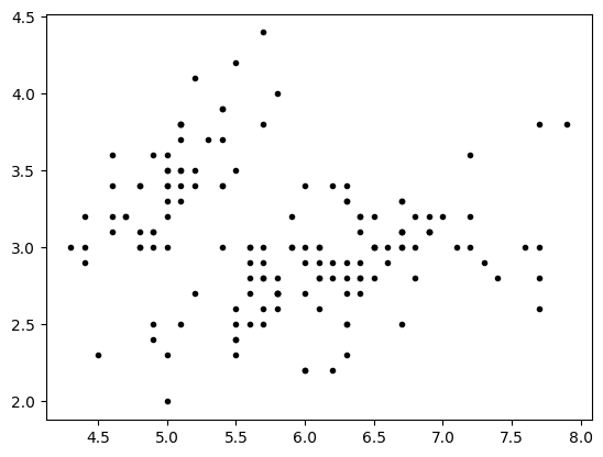
• Unclassified Spatial Mapping: Plotting Sepal Length (sl) vs. Sepal Width (sw) using plain markers ('.k') reveals the raw data structure. This helps verify if the morphological features naturally form distinct clusters before applying any algorithmic boundaries.
• Target Label Mapping (iris.target): Inspecting the ground-truth array to map the multi-class numerical taxonomy:
  • 0: Iris setosa
  • 1: Iris versicolor
  • 2: Iris virginica

This inspection links the visual spatial groups with their mathematical labels, establishing the baseline before data binarization.

sl = iris.data[:, 0:1]
sw = iris.data[:, 1:2]
plt.plot(sl,sw,'.k')
plt.show()

iris.target

array([0, 0, 0, 0, 0, 0, 0, 0, 0, 0, 0, 0, 0, 0, 0, 0, 0, 0, 0, 0, 0, 0,
       0, 0, 0, 0, 0, 0, 0, 0, 0, 0, 0, 0, 0, 0, 0, 0, 0, 0, 0, 0, 0, 0,
       0, 0, 0, 0, 0, 0, 1, 1, 1, 1, 1, 1, 1, 1, 1, 1, 1, 1, 1, 1, 1, 1,
       1, 1, 1, 1, 1, 1, 1, 1, 1, 1, 1, 1, 1, 1, 1, 1, 1, 1, 1, 1, 1, 1,
       1, 1, 1, 1, 1, 1, 1, 1, 1, 1, 1, 1, 2, 2, 2, 2, 2, 2, 2, 2, 2, 2,
       2, 2, 2, 2, 2, 2, 2, 2, 2, 2, 2, 2, 2, 2, 2, 2, 2, 2, 2, 2, 2, 2,
       2, 2, 2, 2, 2, 2, 2, 2, 2, 2, 2, 2, 2, 2, 2, 2, 2, 2])

Step 4: Theoretical Sigmoid Function & Decision Boundary

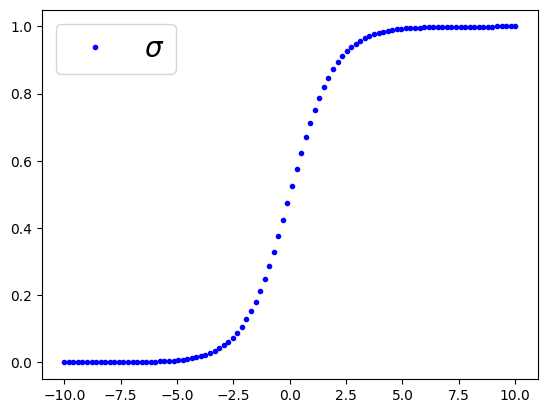
Generating a synthetic domain from -10 to 10 to plot the standalone mathematical Sigmoid function:

\sigma(t) = \frac{1}{1 + e^{-t}}

This visualizes how the curve maps inputs to a probability between 0 and 1, establishing the inflection point \sigma(0) = 0.5 as the theoretical threshold for the decision boundary.

t= np.linspace(-10,10,100)
sig = 1/(1+np.exp(-t))
plt.plot(t,sig, '.b', label=r"$\sigma$")
plt.legend(loc='upper left', fontsize=20)
plt.show()

Model Training and Benchmark Evaluation

Model 1: Iris-Setosa Classifier based on petal width

Feature Selection & Setosa Target Binarization

The dataset is filtered and restructured to evaluate a new binary classification task:

• Feature Vector (X): Slicing index [:, 3:] isolates Petal Width as the continuous predictor variable.
• Target Binarization (y): The criteria (iris.target == 0).astype(int) shifts the positive class (y=1) exclusively to Iris setosa, mapping all other species to 0. This creates the target array seen in the output.

x = iris.data[:, 3:]
y = (iris.target == 0).astype(int)
y

array([1, 1, 1, 1, 1, 1, 1, 1, 1, 1, 1, 1, 1, 1, 1, 1, 1, 1, 1, 1, 1, 1,
       1, 1, 1, 1, 1, 1, 1, 1, 1, 1, 1, 1, 1, 1, 1, 1, 1, 1, 1, 1, 1, 1,
       1, 1, 1, 1, 1, 1, 0, 0, 0, 0, 0, 0, 0, 0, 0, 0, 0, 0, 0, 0, 0, 0,
       0, 0, 0, 0, 0, 0, 0, 0, 0, 0, 0, 0, 0, 0, 0, 0, 0, 0, 0, 0, 0, 0,
       0, 0, 0, 0, 0, 0, 0, 0, 0, 0, 0, 0, 0, 0, 0, 0, 0, 0, 0, 0, 0, 0,
       0, 0, 0, 0, 0, 0, 0, 0, 0, 0, 0, 0, 0, 0, 0, 0, 0, 0, 0, 0, 0, 0,
       0, 0, 0, 0, 0, 0, 0, 0, 0, 0, 0, 0, 0, 0, 0, 0, 0, 0])

Benchmark Model Initialization and Fitting

This cell instantiates and trains the baseline classification model using Scikit-Learn:

• LogisticRegression(solver='lbfgs', random_state=42): Instantiates the model using the Limited-memory BFGS (lbfgs) optimization solver and locks the random_state to 42 to ensure reproducible weight initialization.
• mylr.fit(x, y): Trains the classifier on the isolated feature vector x and the binarized target labels y. This optimization process computes the optimal weight (w) and bias (b) parameters that minimize the loss function.

from sklearn.linear_model import LogisticRegression
mylr = LogisticRegression(solver='lbfgs', random_state=42)
mylr.fit(x,y);

Xnew = np.linspace(-1,3,100).reshape(-1,1)
yPred = mylr.predict_proba(Xnew)
#plt.plot(Xnew, yPred[:,0], label= 'No Iris')
plt.plot(Xnew, yPred[:,1], label= 'Yes Iris')
plt.legend()
plt.plot(x,y,'*g')
plt.show()

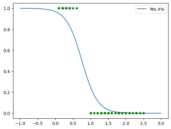
This plot visualizes the trained model's Sigmoid prediction curve over the experimental dataset samples:

• Sample Distribution (Green Stars): Represents the real dataset. Small petal widths (0.1 - 0.6 cm) belong to Iris setosa (y=1), while larger widths (1.0 - 2.5 cm) belong to the other species (y=0).
• Sigmoid Mapping (Blue Curve): Displays an inverted logistic curve. It demonstrates the mathematical relationship: as petal width increases, the probability of the flower being Iris setosa drops sharply from 1.0 to 0.0.
• Decision Boundary Threshold: The curve crosses the 0.5 probability threshold at approximately 0.75 cm. This inflection point defines the exact baseline boundary separating both classifications.

Model 2: Iris-Setosa Classifier based on petal length

Feature Shift – Petal Length Isolation

The model configuration is updated to evaluate a different morphological predictor:

• Feature Vector (X): Slicing index [:, 2:3] isolates Petal Length as the independent variable.
• Target Continuity (y): The classification objective remains focused on Iris setosa (iris.target == 0) to compare the separation power of petal length against the previous petal width baseline.

x = iris.data[:, 2:3]
y = (iris.target == 0).astype(int)

from sklearn.linear_model import LogisticRegression
mylr = LogisticRegression(solver='lbfgs', random_state=42)
mylr.fit(x,y);

Xnew = np.linspace(0,8,100).reshape(-1,1)
yPred = mylr.predict_proba(Xnew)
#plt.plot(Xnew, yPred[:,0], label= 'No Iris')
plt.plot(Xnew, yPred[:,1], label= 'Yes Iris')
plt.legend()
plt.plot(x,y,'*g')
plt.axis([1.5, 5, -0.5, 1.5])
plt.show()

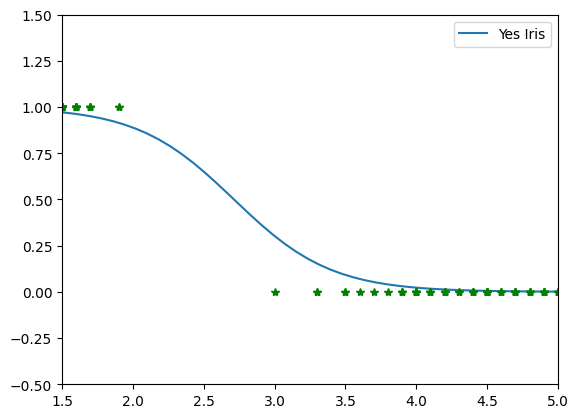
This plot illustrates the performance of the second univariable model using Petal Length:

• Sample Distribution: Samples with short petal lengths (1.0 - 2.0 cm) are correctly clustered as Iris setosa (y=1), while samples with larger lengths (>3.0 cm) map to y=0.
• Sigmoid Mapping: The descending blue curve demonstrates that as petal length increases, the probability of the sample being Iris setosa drops sharply from 1.0 to 0.0.
• Decision Boundary: The curve crosses the 0.5 probability threshold at approximately 2.5 cm, marking the exact inflection point that separates the target class from the rest of the dataset.

Model 3: Iris-Setosa Classifier based on Sepal length

Feature Shift – Sepal Length Isolation

The model evaluates a third morphological predictor independently:

• Feature Vector (X): Slicing index [:, 0:1] isolates Sepal Length as the continuous independent variable.
• Target Continuity (y): The objective remains focused on Iris setosa (y=1) to compare the separation power of sepal dimensions against the previous petal metrics.

x = iris.data[:, 0:1]
y = (iris.target == 0).astype(int)
from sklearn.linear_model import LogisticRegression
mylr = LogisticRegression(solver='lbfgs', random_state=42)
mylr.fit(x,y);

Xnew = np.linspace(0,8,100).reshape(-1,1)
yPred = mylr.predict_proba(Xnew)
#plt.plot(Xnew, yPred[:,0], label= 'No Iris')
plt.plot(Xnew, yPred[:,1], label= 'Yes Iris')
plt.legend()
plt.plot(x,y,'*g')
plt.axis([3.5, 7, -0.1, 1.1])
plt.show()

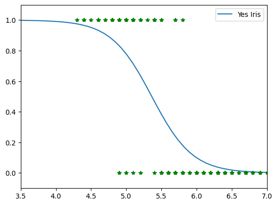
This plot displays the performance of the third univariable model using Sepal Length:

• Sample Distribution: Samples representing Iris setosa (y=1) are concentrated at shorter lengths, but show a much higher spatial overlap with non-setosa samples (y=0) compared to the previous petal features.
• Sigmoid Mapping: The descending curve shows the probability dropping as sepal length increases. Due to this significant data overlap, the slope is less steep, indicating a more gradual and less aggressive probabilistic transition.
• Decision Boundary: The inflection point at \sigma = 0.5 establishes the final threshold. This boundary carries more classification uncertainty because sepal dimensions are naturally less distinct between these species.

Model 4: Multiple features classifier

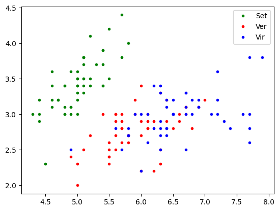
Multi-Class Spatial Mapping (Sepal Features)

This cell upgrades the initial exploratory plot by adding the ground-truth class labels to the 2D sepal feature space:

• Feature Interaction: Maps Sepal Length (sl) against Sepal Width (sw) simultaneously to analyze their combined distribution.
• Class Color-Coding: Differentiates the three original species using distinct markers: Green for Setosa, Red for Versicolor, and Blue for Virginica.
• Visual Separability Analysis: Allows immediate observation of the data structure, showing that while Setosa forms a perfectly isolated cluster, Versicolor and Virginica exhibit significant spatial overlap, justifying the need for optimization models.

import matplotlib.pyplot as plt
sl = iris.data[:,0:1]
sw = iris.data[:,1:2]
tg = iris.target
plt.plot(sl[tg==0,0], sw[tg==0,0],'.g' ,label='Set')
plt.plot(sl[tg==1,0], sw[tg==1,0],'.r', label='Ver')
plt.plot(sl[tg==2,0], sw[tg==2,0],'.b', label='Vir')
plt.legend()
plt.show()

Bivariate Model Training for Iris Virginica

This cell configures and trains a multi-feature logistic regression model utilizing tuned optimization parameters:

• Bivariate Data Selection: * Features (X): Slices index [:, 0:2] to combine Sepal Length and Sepal Width into a two-dimensional feature space.
  • Target (y): Shifts the positive class focus exclusively to Iris virginica (iris.target == 2).
• Hyperparameter Tuning (mylrvir):
  • solver='newton-cg': Uses the Newton-Conjugate Gradient method to compute accurate optimization paths.
  • C=100 & tol=1e-5: Applies high cost (low regularization) to allow a tighter fit to the data, paired with a strict tolerance for precise convergence.
• mylrvir.fit(X, y): Trains the system to find the optimal weight vector w = [w_1, w_2] and bias (b), establishing the multi-variable benchmark line.

X = iris.data[:,0:2]
y = (iris.target==2).astype(int)
mylrvir = LogisticRegression(
    random_state=22,
    tol=1e-5,
    C=100,
    max_iter=100,
    solver='newton-cg'
)
mylrvir.fit(X,y);

Coordinate Grid Generation & Probability Mapping

This block builds the mathematical testing grid used to map out the complete probability landscape:

• np.meshgrid: Generates a dense 100 \times 100 coordinate grid across the sepal feature space (Length: 3–8 cm, Width: 0–6 cm).
• Xnew (np.c_): Flattens and couples the grid matrices into a matrix of 10,000 discrete 2D spatial coordinates.
• predict_proba(Xnew): Evaluates the trained model across the entire grid, computing the continuous probabilities needed to render the decision contours and 3D surfaces.

x0, x1 = np.meshgrid(
    np.linspace(3,8,100).reshape(-1,1),
    np.linspace(0,6,100).reshape(-1,1)
)
Xnew = np.c_[x0.ravel(), x1.ravel()]
yPred = mylrvir.predict_proba(Xnew)

plt.figure(figsize=(10,4))
plt.plot(X[y==0,0], X[y==0,1],'bs',label='No Virg')
plt.plot(X[y==1,0], X[y==1,1],'g^',label='Virginica')
zz=yPred[:,1].reshape(x0.shape)
contour=plt.contour(x0,x1,zz)
plt.clabel(contour, inline=1,fontsize=15)
plt.xlabel("Sepal Length")
plt.ylabel("Sepal Width")
plt.legend()
plt.show()

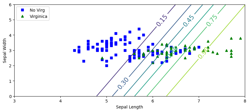
This plot visualizes the continuous probability space generated by the trained bivariate model:

• Sample Distribution: Blue squares represent non-virginica samples (y=0), and green triangles represent Iris virginica (y=1) mapped across Sepal Length and Sepal Width.
• Probability Contours (plt.contour): The labeled contour lines map specific probability thresholds. They show how the model's prediction confidence transitions across the 2D space.
• Decision Boundary: The contour line labeled 0.5 marks the exact geometric threshold. Any sample falling past this line is classified as Iris virginica, capturing the spatial trade-off between both sepal measurements.

fig, ax =plt.subplots(subplot_kw={"projection": "3d"})
surf = ax.plot_surface(x0,x1,zz, cmap='jet')
ax.scatter(iris.data[:,0:1], iris.data[:,1:2], y, 'or');

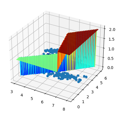
This cell projects the bivariate logistic regression model into a 3D coordinate space to visualize the complete probability landscape:

• Axis Dimensions: The horizontal axes represent Sepal Length (x_1) and Sepal Width (x_2), while the vertical axis (Z) tracks the continuous model probability \sigma(z) \in [0, 1].
• Probability Surface (plot_surface): The Sigmoid function is rendered as a 3D sheet using the jet colormap. It displays the non-linear S-curve transition dynamically stretched across the two-dimensional feature plane.
• True Labels Spatial Scatter (ax.scatter): The red markers plot the actual samples at their exact spatial coordinates and true binary height (z = 1 for Iris virginica, z = 0 for others). This highlights how the optimized surface splits the space to fit the data points.

Modelo 5: Multiple features and muticlass classifier

Multi-Feature & Multi-Class Model Training

This cell configures and trains the final baseline model to handle all three species simultaneously within a two-dimensional feature space:

• Bivariate Inputs (X): Slices index [:, 0:2] to utilize both Sepal Length and Sepal Width as the predictor variables.
• Multi-Class Target (y): Retains the original multi-class target labels (0, 1, 2) without applying binarization, expanding the task from a single boundary to a three-class decision space.
• LogisticRegression(C=100, solver='lbfgs'): Trains a multinomial classifier. The algorithm optimizes a distinct set of weights and biases for each target category, preparing the model to partition the 2D plane into three distinct classification zones.

X = iris.data[:,0:2]
y = iris.target
lrmc = LogisticRegression( 
    solver='lbfgs',
    C=100,
    random_state=22
)
lrmc.fit(X,y);

Multi-Class Grid Generation and Probability Evaluation

This cell sets up the coordinate testing matrix to evaluate the multi-class prediction behavior across the entire sepal feature space:

• np.meshgrid: Constructs a dense 100 \times 100 coordinate grid bounding the Sepal Length (3–8 cm) and Sepal Width (0–6 cm) ranges.
• Xnew (np.c_): Flattens and pairs the grid elements into a matrix of 10,000 distinct 2D spatial coordinates.
• lrmc.predict_proba(Xnew): Computes a three-column probability matrix for each point. This mapping determines the exact multi-class boundaries by evaluating the localized likelihood for Setosa, Versicolor, and Virginica simultaneously.

x0, x1 = np.meshgrid(
    np.linspace(3,8,100).reshape(-1,1),
    np.linspace(0,6,100).reshape(-1,1)
)
Xnew = np.c_[x0.ravel(), x1.ravel()]
yPred = lrmc.predict_proba(Xnew)

plt.figure(figsize=(10,4))
plt.plot(X[y==0,0], X[y==0,1],'.b',label='Setosa')
plt.plot(X[y==1,0], X[y==1,1],'+g',label='Versi')
plt.plot(X[y==2,0], X[y==2,1],'*m',label='Virgi')
zz=yPred[:,1].reshape(x0.shape)
contour=plt.contour(x0,x1,zz)
plt.clabel(contour, inline=1,fontsize=15)
plt.xlabel("Sepal Length")
plt.ylabel("Sepal Width")
plt.legend()
plt.show()

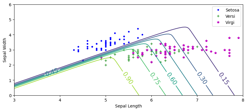
This plot maps the continuous probability distribution of the middle class within the multi-class decision space:

• Three-Class Distribution: Displays all species simultaneously using distinct markers: blue dots for Setosa (y=0), green pluses for Versicolor (y=1), and magenta stars for Virginica (y=2).
• Target Class Extraction (yPred[:, 1]): Slicing the second column of the probability matrix isolates and tracks the specific localized likelihood of a sample being Iris versicolor.
• Localized Probability Ridge: Unlike the linear boundaries seen in binary classification, the multinomial model creates a bounded peak or "ridge" to isolate the middle class. The highest contour line (0.90) tightly encapsulates the core Versicolor cluster, dropping off systematically as the features move toward Setosa (left) or Virginica (right) territories.

yPred = lrmc.predict(Xnew)
plt.figure(figsize=(10,6))
plt.plot(X[y==0,0], X[y==0,1],'bs',label='Setosa')
plt.plot(X[y==1,0], X[y==1,1],'g^',label='Versi')
plt.plot(X[y==2,0], X[y==2,1],'*m',label='Virgi')
zz=yPred.reshape(x0.shape)
contour=plt.contourf(x0,x1,zz, cmap='jet', alpha=0.3)
plt.clabel(contour, inline=1,fontsize=15)
plt.xlabel("Sepal Length")
plt.ylabel("Sepal Width")
plt.legend()
plt.show()

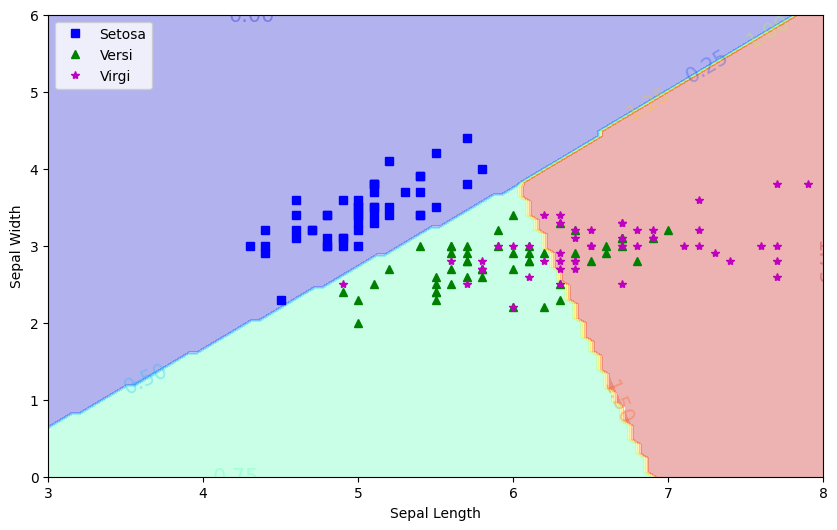
This plot visualizes the ultimate classification boundaries by partitioning the entire 2D feature space into hard decision zones:

• Hard Class Assignment (lrmc.predict): Converts continuous probabilities into discrete class verdicts (0, 1, or 2) by applying an argmax function (selecting the class with the highest probability for each point).
• Filled Decision Regions (plt.contourf): Shades the coordinate plane into three distinct, solid zones using the jet colormap:
  • Blue Region: Absolute classification space for Iris setosa.
  • Green Region: Absolute classification space for Iris versicolor.
  • Red/Orange Region: Absolute classification space for Iris virginica.
• Boundary Analysis: The sharp geometric intersections between the colored blocks define the definitive decision thresholds. This layout explicitly reveals how the linear multi-class model manages the regional trade-offs and handles the spatial overlap between the Versicolor and Virginica samples.

fig, ax =plt.subplots(subplot_kw={"projection": "3d"})
surf = ax.plot_surface(x0,x1,zz, cmap='jet')
ax.scatter(iris.data[:,0:1], iris.data[:,1:2], y, 'or');

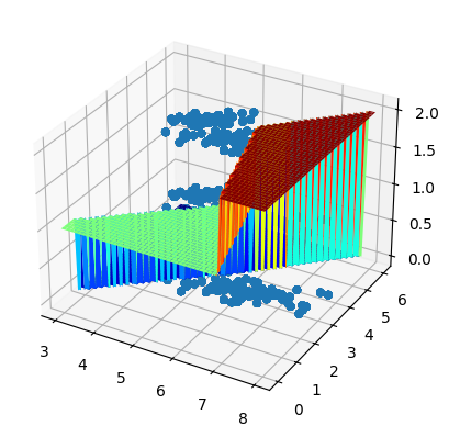
This cell integrates the actual dataset samples into the 3D hard decision space to visually evaluate the multi-class model's accuracy:

• Discrete Vertical Alignment (Z): Both the staircase surface and the scatter markers use the integer multi-class taxonomy (0 for Setosa, 1 for Versicolor, and 2 for Virginica) instead of continuous probabilities.
• Stepped Surface (plot_surface): Represents the geometric boundaries computed by the model. Each level dictates the categorical verdict zone based on the combination of sepal features.
• True Labels Scatter (ax.scatter): Plots the real flower samples at their actual feature coordinates and true species height. This allows immediate visual verification of performance: samples resting on their matching colored step are correctly classified, while those caught on the wrong tier highlight the exact instances of classification error caused by spatial overlap.