2-ne-bgd-25b/Readme.md

Multi-parametric OLS

The multiprarmetric linear regression is a training procedure based on a linear model. The model makes a prediction by simply computing a weighted sum of the input features, plus a constant term called the bias term (also called the intercept term):

 \hat{y}=\theta_0 + \theta_1 x_1 + \theta_2 x_2 + \cdots + \theta_n x_n

This new model includes \theta_n unknown parameter. Thus, the model can be writen more easy by using vector notation form for m instances. Therefore, the model will become in matrix form Y=X\times\theta:

 
\begin{bmatrix} 
    \hat{y}^0 \\ 
    \hat{y}^1\\ 
    \hat{y}^2\\ 
    \vdots \\ 
    \hat{y}^m 
\end{bmatrix} 
= 
\begin{bmatrix} 
    1 & x_1^0 & x_2^0 & \cdots & x_n^0\\ 
    1 & x_1^1 & x_2^1 & \cdots & x_n^1\\
    1 & x_1^2 & x_2^2 & \cdots & x_n^2\\
    \vdots & \vdots & \vdots &\cdots& \vdots\\
    1 & x_0^m & x_1^m & \cdots &x_n^m 
\end{bmatrix} 
\begin{bmatrix} 
    \theta_0 \\ 
    \theta_1 \\ 
    \theta_2 \\ 
    \vdots \\ 
    \theta_n 
\end{bmatrix} 

Resulting:

\hat{y}= h_\theta(x) = x \theta 

Now that we have our model, how do we train it?

Please, consider that training the model means adjusting the parameters to reduce the error or minimizing the cost function. The most common performance measure of a regression model is the Mean Square Error (MSE). Therefore, to train a Linear Regression model, you need to find the value of \theta that minimizes the MSE:

J = MSE(X,h_\theta) = \frac{1}{m} \sum_{i=1}^{m} \left(\hat{y}^{(i)}-y^{(i)} \right)^2

J = MSE(X,h_\theta) = \frac{1}{m} \sum_{i=1}^{m} \left( x^{(i)}\theta-y^{(i)} \right)^2

J = MSE(X,h_\theta) = \frac{1}{m} \left( x\theta-y \right)^T \left( x\theta-y \right)

The normal equation

To find the value of \theta that minimizes the cost function, there is a closed-form solution that gives the result directly. This is called the Normal Equation; and can be find it by derivating the MSE equation as a function of \theta and making it equals to zero:

\hat{\theta} = (X^T X)^{-1} X^{T} y 

import pandas as pd
df =  pd.read_csv('dataset1.csv')
x1 = df['X1']
df

	X1	X2	y
0	3.745401	0.314292	9.247570
1	9.507143	6.364104	16.257728
2	7.319939	3.143560	16.258844
3	5.986585	5.085707	6.359638
4	1.560186	9.075665	-9.739221
...	...	...	...
95	4.937956	3.492096	6.523018
96	5.227328	7.259557	28.761328
97	4.275410	8.971103	-4.306011
98	0.254191	8.870864	-19.500923
99	1.078914	7.798755	-10.525044

100 rows × 3 columns

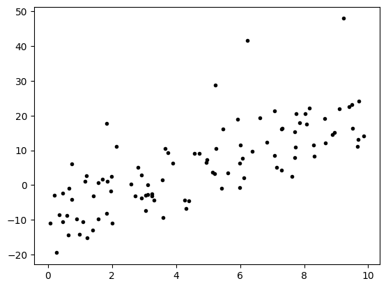
import matplotlib.pyplot as plt
x1 = df['X1']
x2 = df['X2']
y = df['y']
plt.plot(x1,y, '.k')
plt.show()

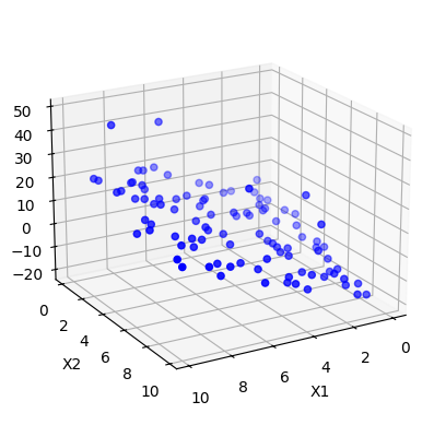
# Create figure and 3D axis
fig = plt.figure()
ax = fig.add_subplot(111, projection='3d')

# Scatter plot
ax.scatter(x1, x2, y, c='blue', marker='o')
ax.view_init(elev=20, azim=60)  # adjust camera

# Axis labels
ax.set_xlabel("X1")
ax.set_ylabel("X2")
ax.set_zlabel("Y")

plt.show()

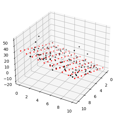
The normal equation

import numpy as np
from numpy.linalg import inv 
x0 = np.ones(len(x1)) 
X = np.c_[x0,x1,x2]
thetaH = np.dot(inv(X.T@X), X.T@y)
thetaH

array([ 0.85319677,  2.98010241, -1.871685  ])

x1New = np.linspace(0,10,10)
x2New= np.linspace(0,10,10)
x1NewG, x2NewG = np.meshgrid(x1New, x2New)
yModel = thetaH[0]+thetaH[1]*x1NewG+thetaH[2]*x2NewG

fig = plt.figure()
ax = fig.add_subplot(111, projection='3d')
ax.scatter(x1NewG, x2NewG, yModel, c='red', marker='.')
ax.scatter(x1, x2, y, c='black', marker='.')
ax.view_init(elev=30, azim=30)  # adjust camera
plt.show()

Batch Gradient Descent

\theta_{new} = \theta_{old}-\eta \nabla_\theta

\nabla_\theta = \frac{2}{m}X^T(X\theta-y)

plt.plot(x1,y, '.k', label="data")
plt.show()

#bgd:
X = np.c_[np.ones_like(x1), x1]
y = np.array(y, ndmin=2).reshape(-1,1)
np.random.seed(67)
n = 1000
m = len(y)
eta = 0.0001
thetaH = np.array([[10],[9]])
thetaH

array([[10],
       [ 9]])

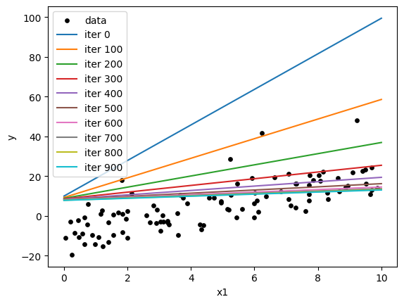
thetaH = np.array([[10],[9]])
x1New = np.linspace(0,10,2)
plt.scatter(x1, y, color="k", s=15, label="data")
#yModel = thetaH[0]+thetaH[1]*x1New
#plt.plot(x1New, yModel, '-g', label="zero")
for iter in range(n):
    nabla = 2/m * X.T@(X@thetaH-y)
    thetaH = thetaH-eta*nabla
    if iter % 100 == 0:
        yModel = thetaH[0]+thetaH[1]*x1New
        plt.plot(x1New,yModel, label=f"iter {iter}")
        print("-=-=-=-=-=-=")
        print(thetaH)
print("Final values:")
print(thetaH) 
plt.xlabel("x1")
plt.ylabel("y")
plt.legend()
plt.show()

-=-=-=-=-=-=
[[9.99064619]
 [8.94558151]]
-=-=-=-=-=-=
[[9.2750177 ]
 [4.93169627]]
-=-=-=-=-=-=
[[8.85060396]
 [2.80897556]]
-=-=-=-=-=-=
[[8.58094375]
 [1.68958788]]
-=-=-=-=-=-=
[[8.39363522]
 [1.10248799]]
-=-=-=-=-=-=
[[8.25026369]
 [0.79775963]]
-=-=-=-=-=-=
[[8.13044659]
 [0.64280814]]
-=-=-=-=-=-=
[[8.02336849]
 [0.56728464]]
-=-=-=-=-=-=
[[7.92328982]
 [0.53386527]]
-=-=-=-=-=-=
[[7.82716409]
 [0.52274774]]
Final values:
[[7.73430322]
 [0.52338189]]

History

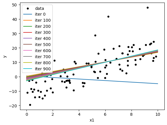
np.random.seed(12)
thetaH = np.random.randn(2,1)
print("Initial values")
print(thetaH)
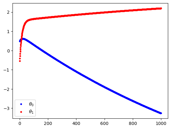
thetas = np.zeros((n,2))
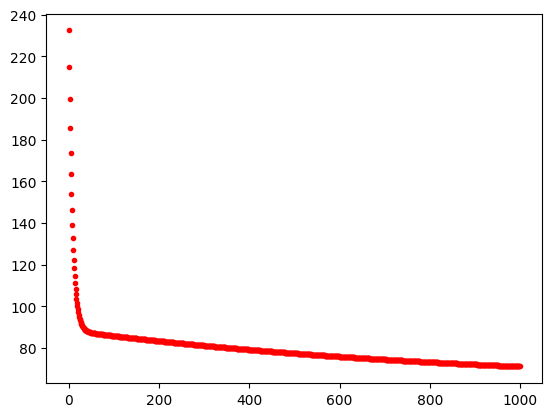
J_hist = np.zeros((n,1))
thetas[0] =  thetaH.ravel()
x1New = np.linspace(0,10,2)
plt.scatter(x1, y, color="k", s=15, label="data")
for iter in range(n):
    nabla = 2/m * X.T@(X@thetaH-y)
    thetaH = thetaH-eta*nabla
    thetas[iter] = thetaH.ravel()
    J = (1/m*(X@thetaH - y).T@(X@thetaH - y))
    # print("J init")
    # print(J)
    J_hist[iter] = J
    if iter % 100 == 0:
        yModel = thetaH[0]+thetaH[1]*x1New
        plt.plot(x1New,yModel, label=f"iter {iter}")
        # print("-=-=-=-=-=-=")
        # print(thetaH)
print("Final values:")
print(thetaH) 
plt.xlabel("x1")
plt.ylabel("y")
plt.legend()
plt.show()

Initial values
[[ 0.47298583]
 [-0.68142588]]
Final values:
[[-3.25986811]
 [ 2.19754312]]

plt.plot(J_hist,'.r')
plt.show

<function matplotlib.pyplot.show(close=None, block=None)>

plt.plot(thetas[:,0], '.b', label=r"$\theta_0$")
plt.plot(thetas[:,1], '.r', label=r"$\theta_1$")
plt.legend()
plt.show()

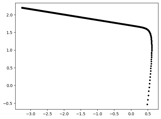
plt.plot(thetas[:,0], thetas[:,1], '.k')
plt.show()

J_hist.shape

(1000, 1)

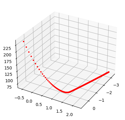
fig = plt.figure()
ax = fig.add_subplot(111, projection='3d')
ax.scatter(thetas[:,0], thetas[:,1], J_hist[:,0], c='red', marker='.')
ax.view_init(elev=30, azim=30)  # adjust camera
plt.show()