You cannot select more than 25 topics
Topics must start with a letter or number, can include dashes ('-') and can be up to 35 characters long.
|
|
3 months ago | |
|---|---|---|
| main_files | 3 months ago | |
| Readme.md | 3 months ago | |
| iris_basic.csv | 4 months ago | |
| main.ipynb | 3 months ago | |
Readme.md
import numpy as np
import pandas as pd
import matplotlib.pyplot as plt
df = pd.read_csv("iris_basic.csv")
print(df.head())
    sl   sw   pl   pw  target  tNames
0  5.1  3.5  1.4  0.2       0  setosa
1  4.9  3.0  1.4  0.2       0  setosa
2  4.7  3.2  1.3  0.2       0  setosa
3  4.6  3.1  1.5  0.2       0  setosa
4  5.0  3.6  1.4  0.2       0  setosa
x = df["pw"].to_numpy().reshape(-1, 1)      # (150,1)
x
array([[0.2],
       [0.2],
       [0.2],
       [0.2],
       [0.2],
       [0.4],
       [0.3],
       [0.2],
       [0.2],
       [0.1],
       [0.2],
       [0.2],
       [0.1],
       [0.1],
       [0.2],
       [0.4],
       [0.4],
       [0.3],
       [0.3],
       [0.3],
       [0.2],
       [0.4],
       [0.2],
       [0.5],
       [0.2],
       [0.2],
       [0.4],
       [0.2],
       [0.2],
       [0.2],
       [0.2],
       [0.4],
       [0.1],
       [0.2],
       [0.2],
       [0.2],
       [0.2],
       [0.1],
       [0.2],
       [0.2],
       [0.3],
       [0.3],
       [0.2],
       [0.6],
       [0.4],
       [0.3],
       [0.2],
       [0.2],
       [0.2],
       [0.2],
       [1.4],
       [1.5],
       [1.5],
       [1.3],
       [1.5],
       [1.3],
       [1.6],
       [1. ],
       [1.3],
       [1.4],
       [1. ],
       [1.5],
       [1. ],
       [1.4],
       [1.3],
       [1.4],
       [1.5],
       [1. ],
       [1.5],
       [1.1],
       [1.8],
       [1.3],
       [1.5],
       [1.2],
       [1.3],
       [1.4],
       [1.4],
       [1.7],
       [1.5],
       [1. ],
       [1.1],
       [1. ],
       [1.2],
       [1.6],
       [1.5],
       [1.6],
       [1.5],
       [1.3],
       [1.3],
       [1.3],
       [1.2],
       [1.4],
       [1.2],
       [1. ],
       [1.3],
       [1.2],
       [1.3],
       [1.3],
       [1.1],
       [1.3],
       [2.5],
       [1.9],
       [2.1],
       [1.8],
       [2.2],
       [2.1],
       [1.7],
       [1.8],
       [1.8],
       [2.5],
       [2. ],
       [1.9],
       [2.1],
       [2. ],
       [2.4],
       [2.3],
       [1.8],
       [2.2],
       [2.3],
       [1.5],
       [2.3],
       [2. ],
       [2. ],
       [1.8],
       [2.1],
       [1.8],
       [1.8],
       [1.8],
       [2.1],
       [1.6],
       [1.9],
       [2. ],
       [2.2],
       [1.5],
       [1.4],
       [2.3],
       [2.4],
       [1.8],
       [1.8],
       [2.1],
       [2.4],
       [2.3],
       [1.9],
       [2.3],
       [2.5],
       [2.3],
       [1.9],
       [2. ],
       [2.3],
       [1.8]])
y = df["target"].to_numpy().reshape(-1, 1)  # (150,1)
y = (y == 0).astype(float)
y
array([[1.],
       [1.],
       [1.],
       [1.],
       [1.],
       [1.],
       [1.],
       [1.],
       [1.],
       [1.],
       [1.],
       [1.],
       [1.],
       [1.],
       [1.],
       [1.],
       [1.],
       [1.],
       [1.],
       [1.],
       [1.],
       [1.],
       [1.],
       [1.],
       [1.],
       [1.],
       [1.],
       [1.],
       [1.],
       [1.],
       [1.],
       [1.],
       [1.],
       [1.],
       [1.],
       [1.],
       [1.],
       [1.],
       [1.],
       [1.],
       [1.],
       [1.],
       [1.],
       [1.],
       [1.],
       [1.],
       [1.],
       [1.],
       [1.],
       [1.],
       [0.],
       [0.],
       [0.],
       [0.],
       [0.],
       [0.],
       [0.],
       [0.],
       [0.],
       [0.],
       [0.],
       [0.],
       [0.],
       [0.],
       [0.],
       [0.],
       [0.],
       [0.],
       [0.],
       [0.],
       [0.],
       [0.],
       [0.],
       [0.],
       [0.],
       [0.],
       [0.],
       [0.],
       [0.],
       [0.],
       [0.],
       [0.],
       [0.],
       [0.],
       [0.],
       [0.],
       [0.],
       [0.],
       [0.],
       [0.],
       [0.],
       [0.],
       [0.],
       [0.],
       [0.],
       [0.],
       [0.],
       [0.],
       [0.],
       [0.],
       [0.],
       [0.],
       [0.],
       [0.],
       [0.],
       [0.],
       [0.],
       [0.],
       [0.],
       [0.],
       [0.],
       [0.],
       [0.],
       [0.],
       [0.],
       [0.],
       [0.],
       [0.],
       [0.],
       [0.],
       [0.],
       [0.],
       [0.],
       [0.],
       [0.],
       [0.],
       [0.],
       [0.],
       [0.],
       [0.],
       [0.],
       [0.],
       [0.],
       [0.],
       [0.],
       [0.],
       [0.],
       [0.],
       [0.],
       [0.],
       [0.],
       [0.],
       [0.],
       [0.],
       [0.],
       [0.],
       [0.],
       [0.],
       [0.],
       [0.]])
def sigmoid(z):
    z = np.clip(z, -500, 500)
    sig = 1.0 / (1.0 + np.exp(-z))
    return sig
def log_loss(y, p, eps=1e-12):
    p = np.clip(p, eps, 1 - eps)
    return -np.mean(y*np.log(p) + (1-y)*np.log(1-p))
lr=0.1
epochs=2000
l2=0.0,
X = np.column_stack([x, np.ones_like(x)])
m = X.shape[0]
theta = np.zeros((2,1))
theta
array([[0.],
       [0.]])
X.T
array([[0.2, 0.2, 0.2, 0.2, 0.2, 0.4, 0.3, 0.2, 0.2, 0.1, 0.2, 0.2, 0.1,
        0.1, 0.2, 0.4, 0.4, 0.3, 0.3, 0.3, 0.2, 0.4, 0.2, 0.5, 0.2, 0.2,
        0.4, 0.2, 0.2, 0.2, 0.2, 0.4, 0.1, 0.2, 0.2, 0.2, 0.2, 0.1, 0.2,
        0.2, 0.3, 0.3, 0.2, 0.6, 0.4, 0.3, 0.2, 0.2, 0.2, 0.2, 1.4, 1.5,
        1.5, 1.3, 1.5, 1.3, 1.6, 1. , 1.3, 1.4, 1. , 1.5, 1. , 1.4, 1.3,
        1.4, 1.5, 1. , 1.5, 1.1, 1.8, 1.3, 1.5, 1.2, 1.3, 1.4, 1.4, 1.7,
        1.5, 1. , 1.1, 1. , 1.2, 1.6, 1.5, 1.6, 1.5, 1.3, 1.3, 1.3, 1.2,
        1.4, 1.2, 1. , 1.3, 1.2, 1.3, 1.3, 1.1, 1.3, 2.5, 1.9, 2.1, 1.8,
        2.2, 2.1, 1.7, 1.8, 1.8, 2.5, 2. , 1.9, 2.1, 2. , 2.4, 2.3, 1.8,
        2.2, 2.3, 1.5, 2.3, 2. , 2. , 1.8, 2.1, 1.8, 1.8, 1.8, 2.1, 1.6,
        1.9, 2. , 2.2, 1.5, 1.4, 2.3, 2.4, 1.8, 1.8, 2.1, 2.4, 2.3, 1.9,
        2.3, 2.5, 2.3, 1.9, 2. , 2.3, 1.8],
       [1. , 1. , 1. , 1. , 1. , 1. , 1. , 1. , 1. , 1. , 1. , 1. , 1. ,
        1. , 1. , 1. , 1. , 1. , 1. , 1. , 1. , 1. , 1. , 1. , 1. , 1. ,
        1. , 1. , 1. , 1. , 1. , 1. , 1. , 1. , 1. , 1. , 1. , 1. , 1. ,
        1. , 1. , 1. , 1. , 1. , 1. , 1. , 1. , 1. , 1. , 1. , 1. , 1. ,
        1. , 1. , 1. , 1. , 1. , 1. , 1. , 1. , 1. , 1. , 1. , 1. , 1. ,
        1. , 1. , 1. , 1. , 1. , 1. , 1. , 1. , 1. , 1. , 1. , 1. , 1. ,
        1. , 1. , 1. , 1. , 1. , 1. , 1. , 1. , 1. , 1. , 1. , 1. , 1. ,
        1. , 1. , 1. , 1. , 1. , 1. , 1. , 1. , 1. , 1. , 1. , 1. , 1. ,
        1. , 1. , 1. , 1. , 1. , 1. , 1. , 1. , 1. , 1. , 1. , 1. , 1. ,
        1. , 1. , 1. , 1. , 1. , 1. , 1. , 1. , 1. , 1. , 1. , 1. , 1. ,
        1. , 1. , 1. , 1. , 1. , 1. , 1. , 1. , 1. , 1. , 1. , 1. , 1. ,
        1. , 1. , 1. , 1. , 1. , 1. , 1. ]])
for i in range(epochs):
    z = X @ theta               # (m,1)
    h = sigmoid(z)              # (m,1)
    grad = (X.T @ (h - y)) / m  # (2,1)  <-- from your formula
    theta -= lr * grad

    #if (i % 0 == 0 or t == epochs-1):
     #   print(f"{i:4d}  loss={log_loss(y, h):.6f}  w={theta[0,0]:.6f}  b={theta[1,0]:.6f}")

w, b = theta[0,0], theta[1,0]
def predict_proba(x, w, b):
    x = np.asarray(x, float).reshape(-1)
    return sigmoid(w*x + b)

def predict(x, w, b, thresh=0.5):
    return (predict_proba(x, w, b) >= thresh).astype(int)
rng = np.random.default_rng(0)
m = 120
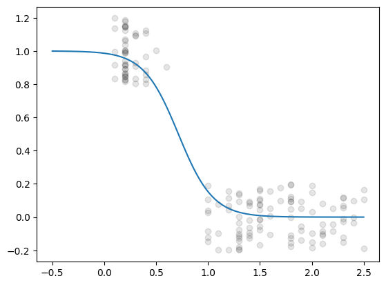
xNew = np.linspace(-0.5, 2.5, m)
p = predict_proba(xNew, w, b)
print(f"\nLearned: w={w:.3f}, b={b:.3f}, loss={log_loss(p.reshape(-1,1), p.reshape(-1,1)):.4f}")
Learned: w=-5.989, b=4.279, loss=0.1812
yJitter = y +np.random.uniform(-0.2, 0.2, size=y.shape)
plt.plot(x, yJitter, 'ok', alpha=0.1)
plt.plot(xNew,p)
[<matplotlib.lines.Line2D at 0x112e5cd70>]
Multi-Parametric Binary Classifier
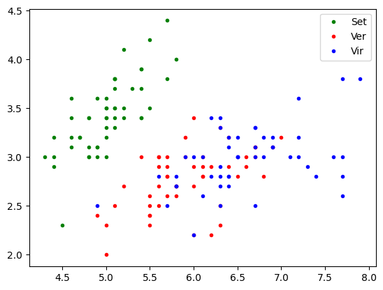
x1 = df["sl"].to_numpy()
x2 = df["sw"].to_numpy()
X = np.column_stack([ np.ones_like(x1), x1, x2])
y = df["target"].to_numpy()
#y = (y == 2).astype(float)
plt.plot(x1[y==0], x2[y==0],'.g' ,label='Set')
plt.plot(x1[y==1], x2[y==1],'.r', label='Ver')
plt.plot(x1[y==2], x2[y==2],'.b', label='Vir')
plt.legend()
plt.show()
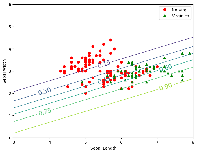
y = df["target"].to_numpy()
y = (y == 2).astype(float)
def predict_proba(X, theta):
    z = X@theta
    return sigmoid(z)
lr=0.01
epochs=5000
m = X.shape[0]
theta = np.random.randn(3)
theta
array([ 0.68799477, 0.14542591, -0.00438461])
for i in range(epochs):
    z = X @ theta               # (m,1)
    h = 1/(1+np.exp(-z))              # (m,1)
    grad = (X.T @ (h - y)) / m  # (2,1)  <-- from your formula
    theta -= lr * grad

    if (i % 100 == 0):
        print(f"{i:4d}  loss={log_loss(y, h):.6f}")

theta
   0  loss=1.178088
 100  loss=0.647786
 200  loss=0.630318
 300  loss=0.615215
 400  loss=0.602111
 500  loss=0.590698
 600  loss=0.580716
 700  loss=0.571949
 800  loss=0.564217
 900  loss=0.557369
1000  loss=0.551279
1100  loss=0.545841
1200  loss=0.540968
1300  loss=0.536583
1400  loss=0.532624
1500  loss=0.529037
1600  loss=0.525776
1700  loss=0.522803
1800  loss=0.520083
1900  loss=0.517587
2000  loss=0.515291
2100  loss=0.513174
2200  loss=0.511214
2300  loss=0.509398
2400  loss=0.507709
2500  loss=0.506136
2600  loss=0.504667
2700  loss=0.503292
2800  loss=0.502002
2900  loss=0.500790
3000  loss=0.499649
3100  loss=0.498572
3200  loss=0.497554
3300  loss=0.496590
3400  loss=0.495676
3500  loss=0.494807
3600  loss=0.493980
3700  loss=0.493191
3800  loss=0.492438
3900  loss=0.491718
4000  loss=0.491028
4100  loss=0.490367
4200  loss=0.489731
4300  loss=0.489120
4400  loss=0.488532
4500  loss=0.487964
4600  loss=0.487416
4700  loss=0.486887
4800  loss=0.486374
4900  loss=0.485877


array([-0.45875015,  1.02970203, -2.10588172])
x1New, x2New = np.meshgrid(
    np.linspace(3,8,100).reshape(-1,1),
    np.linspace(0,6,100).reshape(-1,1))
XNew = np.column_stack([np.ones(x1New.size), x1New.ravel(), x2New.ravel()])

z = XNew @ theta
yPred = 1 / (1 + np.exp(-z))
zz = yPred.reshape(x1New.shape)
zz
array([[9.32789869e-01, 9.35977755e-01, 9.39024319e-01, ...,
        9.99535858e-01, 9.99559369e-01, 9.99581689e-01],
       [9.24332755e-01, 9.27890766e-01, 9.31293909e-01, ...,
        9.99472707e-01, 9.99499415e-01, 9.99524770e-01],
       [9.14908551e-01, 9.18870810e-01, 9.22664164e-01, ...,
        9.99400969e-01, 9.99431308e-01, 9.99460111e-01],
       ...,
       [5.83101559e-05, 6.14226291e-05, 6.47012289e-05, ...,
        8.96718270e-03, 9.44134205e-03, 9.94032212e-03],
       [5.13237738e-05, 5.40633488e-05, 5.69491493e-05, ...,
        7.90122160e-03, 8.31948909e-03, 8.75970294e-03],
       [4.51744213e-05, 4.75857700e-05, 5.01258268e-05, ...,
        6.96108505e-03, 7.32995218e-03, 7.71821361e-03]], shape=(100, 100))
plt.figure(figsize=(8,6))
plt.plot(x1[y==0], x2[y==0],'or' ,label='No Virg')
plt.plot(x1[y==1], x2[y==1],'g^',label='Virginica')
contour = plt.contour(x1New,x2New,zz, linewidths=1)
plt.clabel(contour, inline=1,fontsize=15)
plt.xlabel("Sepal Length")
plt.ylabel("Sepal Width")
plt.legend()
plt.show()
# Softmax model ???