Gerardo Marx
5aada84c7c
Gerardo Marx
5aada84c7c
|
6 years ago | |
|---|---|---|
| .gitignore | 6 years ago | |
| Poisson.ipynb | 6 years ago | |
| Readme.md | 6 years ago | |
| output_6_0.png | 6 years ago | |
| output_8_0.png | 6 years ago | |
| paraview-results.png | 6 years ago | |
| physicalproblem.PNG | 6 years ago | |
| resulteq.png | 6 years ago | |
| solution.pvd | 6 years ago | |


Readme.md
Introduction
The Poisson's equation is a second-order partial differential equation that stats the negative Laplacian -\Delta u of an unknown field u=u(x) is equal to a given function f=f(x) on a domain \Omega \subset \mathbb{R}^d, most probably defined by a set of boundary conditions for the solution u on the boundary \partial \Omega of \Omega:
-\Delta u =f \quad \text{in } \Omega\text{,}u=u_0 \quad \text{on } \Gamma_D \subset \partial\Omega \text{,}here the Dirichlet's boundary condition u=u_0 signifies a prescribed values for the unknown u on the boundary.
The Poisson's equation is the simplest model for gravity, electromagnetism, heat transfer, among others.
The specific case of f=0 and a negative k value, leaves to the Fourier's Law.
Comparative analysis
Along this example, the fenics platfomr is used to compare results obtained by solving the heat equation (Laplace equation) in 2-D:
\frac{\partial^2 T}{\partial x^2}+ \frac{\partial^2 T}{\partial y^2}=0the problem is defined by the next geometry considerations:

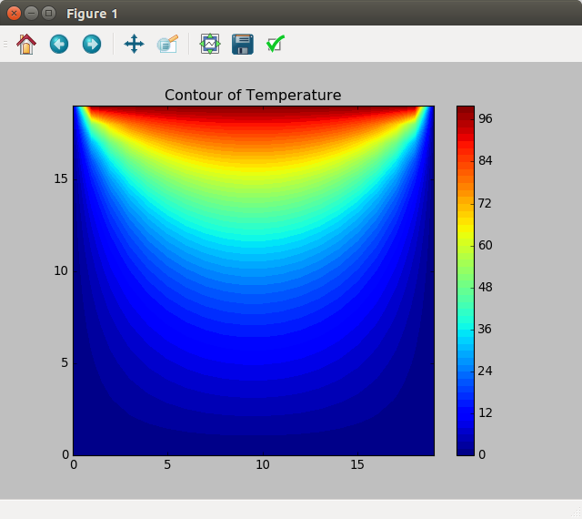
The resulting contour of temperature, solving using finite diferences, is shown next:
Solving by Finite Element Method with Varational Problem formulation
#1 Loading functions  and modules
from fenics import *
import matplotlib.pyplot as plt
#2 Create mesh and define function space
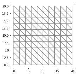
mesh = RectangleMesh(Point(0,0),Point(20,20),10, 10,'left')
V = FunctionSpace(mesh, 'Lagrange', 1) #Lagrange are triangular elements
plot(mesh)
plt.show()
#3 Defining boundary conditions (Dirichlet)
tol = 1E-14 # tolerance for coordinate comparisons
#at y=20
def Dirichlet_boundary1(x, on_boundary):
    return on_boundary and abs(x[1] - 20) < tol
#at y=0
def Dirichlet_boundary0(x, on_boundary):
    return on_boundary and abs(x[1] - 0) < tol
#at x=0
def Dirichlet_boundarx0(x, on_boundary):
    return on_boundary and abs(x[0] - 0) < tol
#at x=20
def Dirichlet_boundarx1(x, on_boundary):
    return on_boundary and abs(x[0] - 20) < tol

bc0 = DirichletBC(V, Constant(0), Dirichlet_boundary0)
bc1 = DirichletBC(V, Constant(100), Dirichlet_boundary1) #100C
bc2 = DirichletBC(V, Constant(0), Dirichlet_boundarx0)
bc3 = DirichletBC(V, Constant(0), Dirichlet_boundarx1)
bcs = [bc0,bc1, bc2,bc3]
#4 Defining variational problem and its solution
k =1
u = TrialFunction(V)
v = TestFunction(V)
f = Constant(0)
a = dot(k*grad(u), grad(v))*dx
L = f*v*dx

# Compute solution
u = Function(V)
solve(a == L, u, bcs)

# Plot solution and mesh
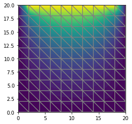
plot(u)
plot(mesh)

# Save solution to file in VTK format
vtkfile = File('solution.pvd')
vtkfile << u
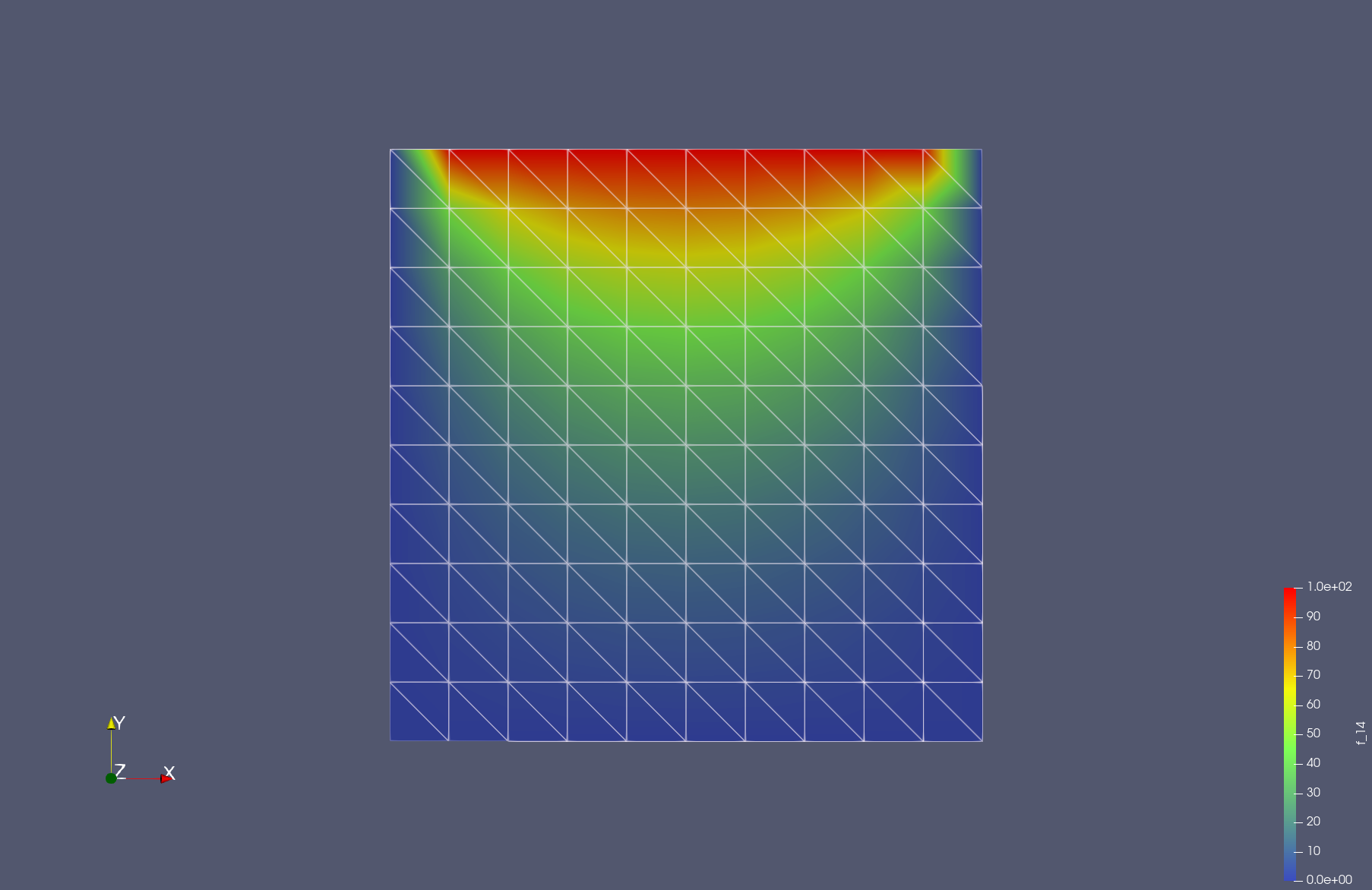
Results after editing color-map on paraview