5-ann-tf-demo-session/Readme.md

#!pip3 install tensorflow
import tensorflow as tf
import numpy as np
import matplotlib.pyplot as plt

# data for training the ann mode
# option 1:
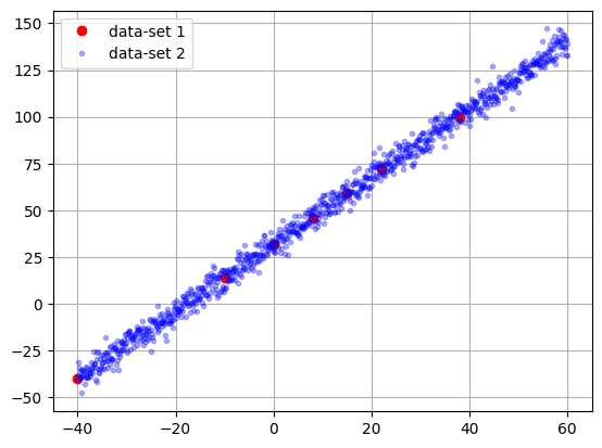
celsius = np.array([-40, -10, 0, 8, 15, 22, 38], dtype=float)
fahrenheit = np.array([-40, 14, 32, 46, 59, 72, 100], dtype=float)

# option 2: (X°C x 9/5) + 32 = 41 °F
points = 1000
np.random.seed(99)
dataIn = np.linspace (-40,60, points)
target = dataIn*9/5 + 32 +4*np.random.randn(points)

plt.plot(celsius, fahrenheit, 'or', label='data-set 1')
plt.plot(dataIn, target, '.b', alpha=0.3, label='data-set 2')
plt.legend()
plt.grid()
plt.show()

from tensorflow.keras.models import Sequential # ANN type
from tensorflow.keras.layers import Dense, Input # All nodes connected

# NN definition
hn=2
model = Sequential()
model.add(Input(shape=(1,), name='input'))
model.add(Dense(hn, activation='linear', name='hidden'))
model.add(Dense(1, activation='linear', name='output'))
model.summary()

Model: "sequential_1"

┏━━━━━━━━━━━━━━━━━━━━━━━━━━━━━━━━━┳━━━━━━━━━━━━━━━━━━━━━━━━┳━━━━━━━━━━━━━━━┓
┃ Layer (type)                    ┃ Output Shape           ┃       Param # ┃
┡━━━━━━━━━━━━━━━━━━━━━━━━━━━━━━━━━╇━━━━━━━━━━━━━━━━━━━━━━━━╇━━━━━━━━━━━━━━━┩
│ hidden (Dense)                  │ (None, 2)              │             4 │
├─────────────────────────────────┼────────────────────────┼───────────────┤
│ output (Dense)                  │ (None, 1)              │             3 │
└─────────────────────────────────┴────────────────────────┴───────────────┘

 Total params: 7 (28.00 B)

 Trainable params: 7 (28.00 B)

 Non-trainable params: 0 (0.00 B)

### veri important note implement a python code 
# to show the ANN model connection using ascii

from tensorflow.keras.optimizers import Adam

#hyper parameters
epoch = 500
lr = 0.01
tf.random.set_seed(99)  # For TensorFlow


model.compile(optimizer=Adam(lr), loss='mean_squared_error')
print("Starting training ...")
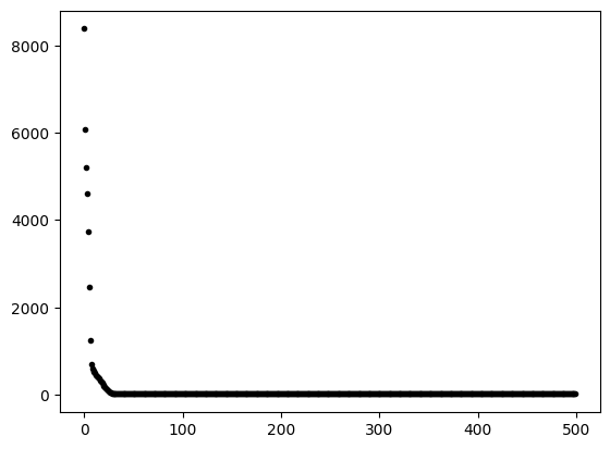
historial = model.fit(dataIn, target, epochs=epoch, verbose=False,)
print("Model trainned!")

Starting training ...
Model trainned!

plt.plot(historial.epoch, historial.history['loss'], '.k' )
plt.show()

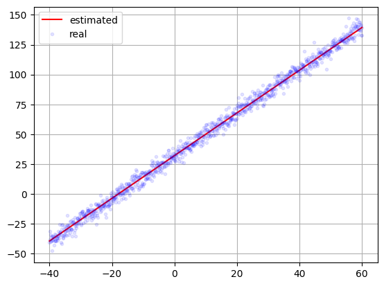
predict = model.predict(dataIn)
plt.plot(dataIn, predict, '-r', label='estimated')
plt.plot(dataIn,target, '.b', label='real', alpha=0.1)
#plt.xlim([0, 20])
#plt.ylim([32, 39])
plt.legend()
plt.grid()
plt.show()

32/32 ━━━━━━━━━━━━━━━━━━━━ 0s 741us/step

for layer in model.layers:
    print(layer.get_weights())

[array([[ 0.7760521 , -0.18955402]], dtype=float32), array([8.428659, 8.034532], dtype=float32)]
[array([[2.4613197 ],
       [0.63733613]], dtype=float32), array([6.2560296], dtype=float32)]

# Get weights
for layer in model.layers:
    weights = layer.get_weights()
    print(f"Layer: {layer.name}")
    print(f"  Weights (Kernel): {weights[0].shape} \n{weights[0]}")
    print(f"  Biases: {weights[1].shape} \n{weights[1]}")

Layer: hidden
  Weights (Kernel): (1, 2) 
[[ 0.7760521  -0.18955402]]
  Biases: (2,) 
[8.428659 8.034532]
Layer: output
  Weights (Kernel): (2, 1) 
[[2.4613197 ]
 [0.63733613]]
  Biases: (1,) 
[6.2560296]

inData = np.array([100])
model.predict(inData)

1/1 ━━━━━━━━━━━━━━━━━━━━ 0s 25ms/step





array([[211.05261]], dtype=float32)

wih = np.array([[ 0.7760521,  -0.18955402]])
bh = np.array([8.428659, 8.034532])
Xh = np.dot(inData, wih) + bh
who = np.array([[2.4613197 ],[0.63733613]])
bo = np.array([6.2560296])
O = np.dot(Xh,who) + bo
O

array([211.05262121])

Testing the model

inTest = np.array([100])
model.predict(inTest)

1/1 ━━━━━━━━━━━━━━━━━━━━ 0s 22ms/step





array([[115.929985]], dtype=float32)

# Do the Maths:
inTest = np.array(inTest)
whi = np.array([[-0.27738443, 0.7908125 ]])
bh = np.array([-8.219968, 6.714554])
Oh = np.dot(inTest,whi)+bh
who = np.array([[-1.9934888],[ 1.5958738]])
bo = np.array([5.1361823])
Oo = np.dot(Oh,who)+bo
Oo

array([213.73814765])

sklearn

from sklearn.neural_network import MLPRegressor
from sklearn.preprocessing import StandardScaler
from sklearn.model_selection import train_test_split
import numpy as np

# Datos de ejemplo


# Escalado de los datos
scaler_X = StandardScaler()
scaler_y = StandardScaler()

X_scaled = scaler_X.fit_transform(dataIn.reshape(-1,1))
y_scaled = scaler_y.fit_transform(target.reshape(-1, 1)).ravel()

# Modelo equivalente al de Keras
mlp = MLPRegressor(
    hidden_layer_sizes=(2,),     # 1 capa oculta con 2 neuronas
    activation='identity',       # activación lineal
    learning_rate_init=0.001,  # 👈 Learning rate
    solver='adam',
    max_iter=1000,
    tol=1e-6,
    random_state=4
)

# Entrenar modelo
mlp.fit(X_scaled, y_scaled)

# Predicción
y_pred_scaled = mlp.predict(X_scaled)
y_pred = scaler_y.inverse_transform(y_pred_scaled.reshape(-1, 1))

# Visualizar resultados (opcional)
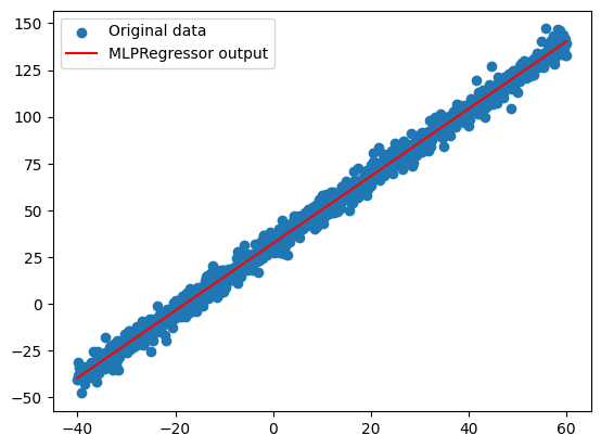
import matplotlib.pyplot as plt

plt.scatter(dataIn, target, label="Original data")
plt.plot(dataIn, y_pred, color='red', label="MLPRegressor output")
plt.legend()
plt.show()

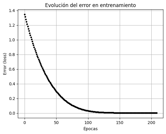
plt.plot(mlp.loss_curve_,'.k')
plt.xlabel("Épocas")
plt.ylabel("Error (loss)")
plt.title("Evolución del error en entrenamiento")
plt.grid(True)
plt.show()

print("Pesos entre capa de entrada y oculta:", mlp.coefs_[0])
print("Pesos entre capa oculta y salida:", mlp.coefs_[1])
print("Bias de capa oculta:", mlp.intercepts_[0])
print("Bias de salida:", mlp.intercepts_[1])

Pesos entre capa de entrada y oculta: [[ 1.70549238 -0.37235861]]
Pesos entre capa oculta y salida: [[ 0.30934654]
 [-1.25842791]]
Bias de capa oculta: [1.02819949 1.02732046]
Bias de salida: [0.97683886]

Model scheme

def generate_ascii_ann(model):
    ascii_diagram = "\nArtificial Neural Network Architecture:\n"
    
    for i, layer in enumerate(model.layers):
        weights = layer.get_weights()
        
        # Determine layer type and number of neurons
        if isinstance(layer, Dense):
            input_dim = weights[0].shape[0]  # Number of inputs
            output_dim = weights[0].shape[1]  # Number of neurons
            
            ascii_diagram += f"\nLayer {i+1}: {layer.name} ({layer.__class__.__name__})\n"
            ascii_diagram += f"  Inputs: {input_dim}, Neurons: {output_dim}\n"
            ascii_diagram += f"  Weights Shape: {weights[0].shape}\n"

            if len(weights) > 1:  # If bias exists
                ascii_diagram += f"  Biases Shape: {weights[1].shape}\n"

            # ASCII representation of neurons
            ascii_diagram += "  " + " o " * output_dim + "  <- Output Neurons\n"
            ascii_diagram += "   |   " * output_dim + "\n"
            ascii_diagram += "  " + " | " * input_dim + "  <- Inputs\n"

    return ascii_diagram

# Generate and print the ASCII diagram
ascii_ann = generate_ascii_ann(model)
print(ascii_ann)

Artificial Neural Network Architecture:

Layer 1: hidden (Dense)
  Inputs: 1, Neurons: 2
  Weights Shape: (1, 2)
  Biases Shape: (2,)
   o  o   <- Output Neurons
   |      |   
   |   <- Inputs

Layer 2: output (Dense)
  Inputs: 2, Neurons: 1
  Weights Shape: (2, 1)
  Biases Shape: (1,)
   o   <- Output Neurons
   |   
   |  |   <- Inputs

graph LR
I1((I_1)) --> H1((H_1))  & H2((H_1))
H1 & H2 --> O1((O_1)) & O2((O_2))