ols-video/main.md

Ordinary Least Squares

Introduction

The Ordinary Least Squares (OLS) is an important method in machine learning and statistics for several reasons. The OLS is a straightforward and easy-to-understand method for fitting linear models.

The model minimizes the sum of squared differences between the observed y and predicted values \hat{y}, making it intuitive to understand.

Additionally, the OLS is the foundation for linear regression, one of the most widely used machine learning and statistics techniques. Linear regression is valuable for modeling relationships between variables when you suspect a linear relationship exists.

While OLS is valuable in many scenarios, it's essential to acknowledge its limitations, especially when dealing with nonlinear relationships or complex data structures.

More advanced machine learning techniques like decision trees, neural networks, or support vector machines may be more appropriate in such cases. However, OLS remains a foundational method with enduring relevance in machine learning and statistics.

Obtaining the OLS general equation

The OLS general model \hat{y} is defined by:

 \hat{y} = \theta_0+\theta_1 x_1 

Applying the partial derivatives with rescpect \theta_0 and equaliting to zero:

\frac{\partial SSR(\theta_0, \theta_1)}{\partial \theta_0}=0 

here SSR is defined as:

 \sum_{i=1}^n (y^i - \hat{y}^i)^2 

Resulting in:

 \theta_0 = \frac{\sum_{i=1}^n y^i}{n} - \frac{\theta_1 \sum_{i=1}^n x^i}{n}

or

 \theta_0 = \bar{y} -\theta_1 \bar{x} 

In a similar way, the partial derivative of SSR with respect of \theta_1 will result in:

\theta_1 = \frac{\sum_{i=1}^n x^i(y^i-\bar{y}) }{\sum_{i=1}^n x^i(x^i-\bar{x})}

Implementing OLS in Python

import numpy as np
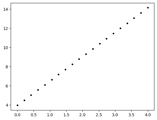
x = np.linspace(0,4,20)
theta0 = 3.9654
theta1 = 2.5456
y = theta0+theta1*x
y

array([ 3.9654    ,  4.50131579,  5.03723158,  5.57314737,  6.10906316,
        6.64497895,  7.18089474,  7.71681053,  8.25272632,  8.78864211,
        9.32455789,  9.86047368, 10.39638947, 10.93230526, 11.46822105,
       12.00413684, 12.54005263, 13.07596842, 13.61188421, 14.1478    ])

import matplotlib.pyplot as plt 
plt.plot(x,y, '.k')
plt.show()

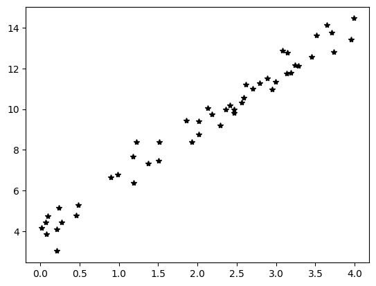
x = 4*np.random.rand(50, 1)
y = theta0 + theta1*x+0.5*np.random.randn(50, 1)
plt.plot(x,y, '*k')
plt.show()

Implementing with for

\theta_1 = \frac{\sum_{i=1}^n x^i(y^i-\bar{y}) }{\sum_{i=1}^n x^i(x^i-\bar{x})}

# for implementation for computing theta1:
xAve = x.mean()
yAve = y.mean()
num = 0
den = 0
for i in range(len(x)):
    num = num + x[i]*(y[i]-yAve)
    den = den + x[i]*(x[i]-xAve)
theta1Hat = num/den
print(theta1Hat)

[2.56763627]

# for implementation for theta0:
# $$ \theta_0 = \bar{y} -\theta_1 \bar{x} $$
theta0Hat = yAve - theta1Hat*xAve
print(theta0Hat)
#real values are
#theta0 = 3.9654
#theta1 = 2.5456

[3.99216691]

total = 0
for i in range(len(x)):
    total = total + x[i]
total/len(x)

array([2.06512069])

Implementing OLS by numpy methods

# For theta1:
# $$\theta_1 = \frac{\sum_{i=1}^n x^i(y^i-\bar{y}) }{\sum_{i=1}^n x^i(x^i-\bar{x})}$$
num2 = np.sum(x*(y-y.mean()))
den2 = np.sum(x*(x-x.mean()))
theta1Hat2 = num2/den2
print(theta1Hat2)

# Efficacy --> time

2.5676362738874774

theta0Hat2 = yAve-theta1Hat2*xAve
theta0Hat2

np.float64(3.992166911745958)

Comparing Model and Data

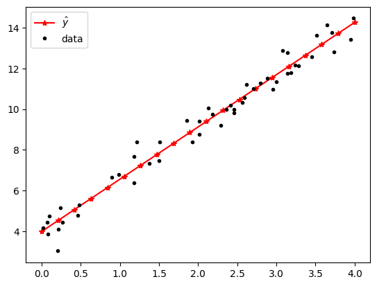
xNew = np.linspace(0,4,20)
yHat = theta0Hat + theta1Hat*xNew
plt.plot(xNew, yHat, '-*r', label="$\hat{y}$")
plt.plot(x,y,'.k', label="data")
plt.legend()
plt.show()

Functions for data and OLS

def DataGen(xn: float,n: int, disp,theta0=3.9654,theta1=2.5456):
    x = xn*np.random.rand(n, 1)
    #theta0 = 3.9654
    #theta1 = 2.5456
    y = theta0+theta1*x+disp*np.random.randn(n,1)
    return x,y

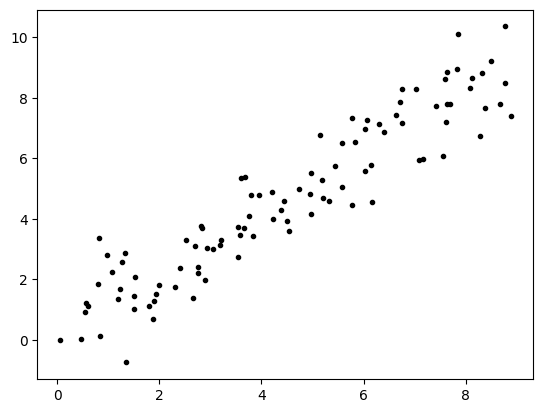
x,y = DataGen(9, 100, 1, 0,1)

plt.plot(x,y,'.k')
plt.show()

def MyOLS(x,y):
    # for implementation for computing theta1:
    xAve = x.mean()
    yAve = y.mean()
    num = 0
    den = 0
    for i in range(len(x)):
        num = num + x[i]*(y[i]-yAve)
        den = den + x[i]*(x[i]-xAve)
    theta1Hat = num/den
    theta0Hat = yAve - theta1Hat*xAve
    return theta0Hat, theta1Hat

the0, the1 = MyOLS(x,y)
the1

array([0.99109086])